Category Archives: Computer Science

Prim’s Algorithm

August 19, 2020algorithms, Computer Scienceadmin

ref –

https://www.geeksforgeeks.org/travelling-salesman-problem-set-2-approximate-using-mst/
https://iq.opengenus.org/graph-representation-adjacency-matrix-adjacency-list/
https://www.gatevidyalay.com/prims-algorithm-prim-algorithm-example/
source – https://github.com/redmacdev1988/PrimsAlgorithm
https://www.tutorialspoint.com/Prim-s-algorithm-in-Javascript

What it solves:

Traveling Salesman Problem (Approximate using Minimum Spanning Tree)

Algorithm:
1) Let 1 be the starting and ending point for salesman.
2) Construct MST from with 1 as root using Prim’s Algorithm.
3) List vertices visited in preorder walk of the constructed MST, and add 1 at the end.

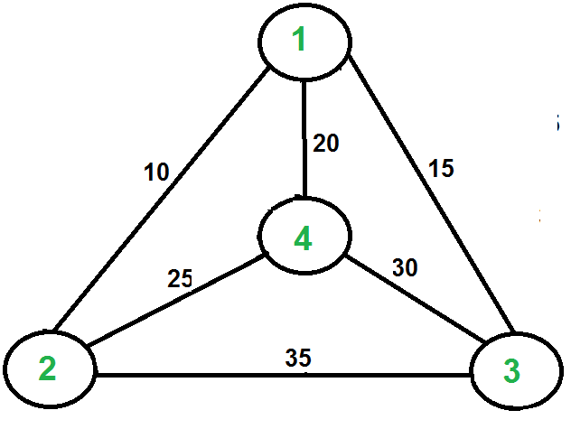
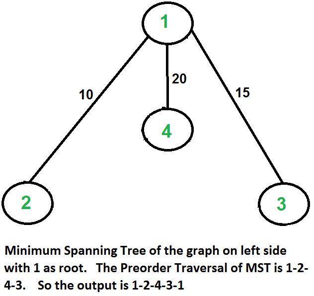
Let us consider the following example. The first diagram is the given graph. The second diagram shows MST constructed with 1 as root. The preorder traversal of MST is 1-2-4-3. Adding 1 at the end gives 1-2-4-3-1 which is the output of this algorithm.

Given a problem like so, we use Prim’s algorithm to create a minimum spanning tree for a weighted undirected graph. It finds a subset of the edges that forms a tree, where the total weight of all the edges in the tree is minimized.

What is Minimum Spanning Tree?

Given a connected and undirected graph, a spanning tree of that graph is a subgraph that is a tree and connects all the vertices together. A single graph can have many different spanning trees. A minimum spanning tree (MST) or minimum weight spanning tree for a weighted, connected and undirected graph is a spanning tree with weight less than or equal to the weight of every other spanning tree. The weight of a spanning tree is the sum of weights given to each edge of the spanning tree.

Prim’s Algorithm

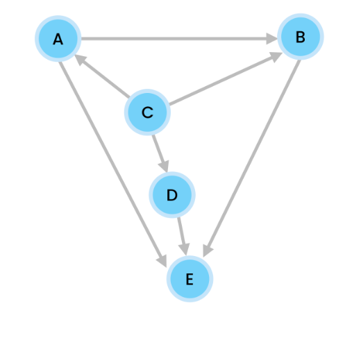
Given Problem

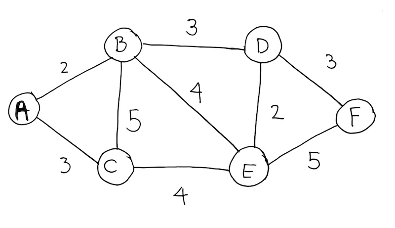
Adjacency List

We create an adjacency list. From the diagram, we see that A connects to B and C. So we create key A, and then have it reference a Linked List with nodes B and C.

We see B connects to C, E, and D. So in our adjacency list, we add key B, and have it reference a Linked List with nodes C, E, and D. Repeat until all edges and vertices have been added.

A -> [B] -> [C]
B -> [A] -> [C] -> [E] -> [D]
C -> [A] -> [B] -> [E]
D -> [B] -> [E] -> [F]
E -> [D] -> [E]

The key to picking only the minimum path and getting rid of the rest is accomplished by:

minimum priority queue
visited dictionary to keep track of all visited nodes

The Minimum Queue

We use the minimum priority queue to keep all the edges from nodes that we have visited. We group these edges into this queue, then take the minimum of it. That is how this algorithm picks the minimum path to travel.

Start

We start at node A so we draw it.

We need to process this node A in our min priority queue so we should add it to initialize our queue.

Min Queue: [A]
Visited: {}

Now that the queue has an item, we can start off the process it.

We pop A from the queue to process it.

Min Queue: []
Visited: {}

Has it been visited? No, so we put it in Visited dictionary.
We see from the adjacency list that A connects to B (with distance of 2) and C (with distance of 3).
So we push B and C into our queue.

Min Queue: [ B(A, 2), C(A, 3) ]
Visited: { “A” }

This means that all edges from A is only B and C. And from this group of edges, we use the min priority queue to get the absolute minimum path (which is 2) at node B.

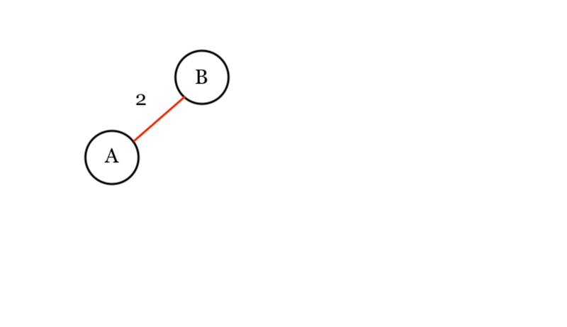
Hence pop B from the queue.

Min Queue: [ C(A, 3) ]
Visited: { “A” }

Has B been visited? We look at the Visited dictionary. No. So we then add B to the visited dictionary. . We draw our result:

So we get all its edges from the adjacency list. We see that its nodes D(B, 3), C(B, 5), and E(B, 4).

Min Queue: [ C(A, 3), D(B, 3), C(B, 5), E(B, 4) ]
Visited: { “A”, “B” }

Now we see that the number of available paths have increased to four. We then get the minimum path, which is C(A,3). Has C been visited? Nope, we add it to the Visited dictionary. We draw the path in our diagram.

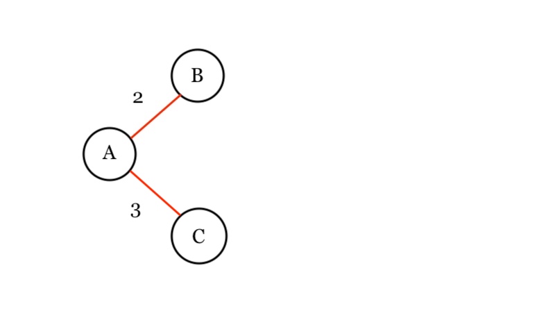
Then we process it by getting all its edges from the adjacency list. We see that it has node of E(C, 4). We push it onto the Min Queue.
Now, we have 4 available paths from nodes A, B, and C.

Min Queue: [ D(B, 3), C(B, 5), E(B, 4), E(C, 4) ]
Visited: { “A”, “B”, “C” }

We get minimum of those paths which is D(B,3). Has D been visited? Nope, we add it to the visited dictionary. We draw the path in our diagram.

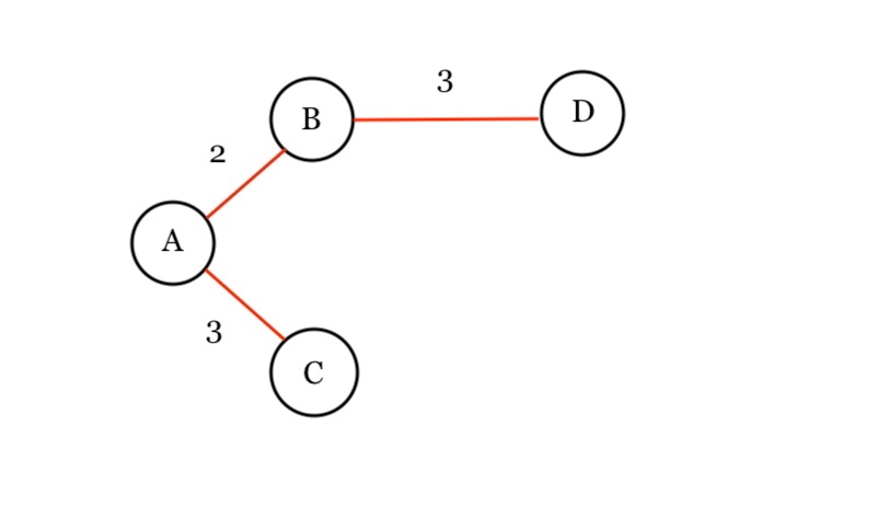
Then we process D by getting all its edges from the adjacency list. We see that it has node of E(D, 2), F(D, 3). We push it onto the Min Queue.

Min Queue: [ C(B, 5), E(B, 4), E(C, 4), E(D, 2), F(D,3) ]
Visited: { “A”, “B”, “C”, “D” }

We pop the minimum of the priority queue: E(D, 2). Has E been visited? Nope, we add it to the visited dictionary. We draw the path in our diagram.

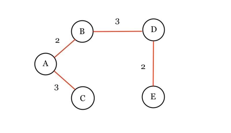
Then we process E by getting all its edges from the adjacency list. We see that it has node of E(F, 5). We push it onto the Min Queue.

Hence at this point, we have 5 available edges from our visited nodes.

Min Queue: [ C(B, 5), E(B, 4), E(C, 4), F(D,3), E(F, 5) ]
Visited: { “A”, “B”, “C”, “D”, “E” }

We pop the minimum which is F(D, 3), and process it. Has F been visited? Nope, we add it to the visited dictionary. We update our answer diagram:

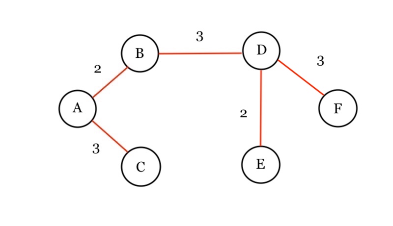
From our adjacency list, we see that F does not have a Linked list of edges. Hence, we DO NOT PUSH ANYTHING onto our Priority Queue:

Min Queue: [ C(B, 5), E(B, 4), E(C, 4), E(F, 5) ]
Visited: { “A”, “B”, “C”, “D”, “E”, “F” }

We keep processing. We pop from the minimum queue: E(B, 4) . Has it been visited? Yes, so we skip and continue dequeueing.

Min Queue: [ C(B, 5), E(C, 4), E(F, 5) ]
Visited: { “A”, “B”, “C”, “D”, “E”, “F” }

We pop from the minimum queue: E(C, 4) . Has it been visited? Yes, so we skip and continue dequeueing.

Min Queue: [ C(B, 5), E(F, 5) ]
Visited: { “A”, “B”, “C”, “D”, “E”, “F” }

We pop from the minimum queue: C(B, 5) . Has it been visited? Yes, so we skip and continue dequeueing.

Min Queue: [ E(F, 5) ]
Visited: { “A”, “B”, “C”, “D”, “E”, “F” }

We pop from the minimum queue: E(F, 5) . Has it been visited? Yes, so we skip it and continue.

Now our queue is empty and we’re done.

The answer is:

Graphs Problems (networks, routes/paths, scheduling…etc)

August 12, 2020algorithms, Computer Scienceadmin

ref –

https://www.geeksforgeeks.org/depth-first-search-or-dfs-for-a-graph/
https://www.geeksforgeeks.org/breadth-first-search-or-bfs-for-a-graph/
https://stackoverflow.com/questions/14720691/whats-the-purpose-of-bfs-and-dfs

BFS and DFS are graph search algorithms that can be used for a variety of different purposes. Many problems in computer science can be thought of in terms of graphs. For example, analyzing networks, mapping routes, and scheduling are graph problems. Graph search algorithms like breadth-first search are useful for analyzing and solving graph problems.

One common application of the two search techniques is to identify all nodes that are reachable from a given starting node. For example, suppose that you have a collection of computers that each are networked to a handful of other computers. By running a BFS or DFS from a given node, you will discover all other computers in the network that the original computer is capable of directly or indirectly talking to. These are the computers that come back marked.

BFS specifically can be used to find the shortest path between two nodes in an unweighted graph. Suppose, for example, that you want to send a packet from one computer in a network to another, and that the computers aren’t directly connected to one another. Along what route should you send the packet to get it to arrive at the destination as quickly as possible? If you run a BFS and at each iteration have each node store a pointer to its “parent” node, you will end up finding route from the start node to each other node in the graph that minimizes the number of links that have to be traversed to reach the destination computer.

DFS is often used as a subroutine in more complex algorithms. For example, Tarjan’s algorithm for computing strongly-connected components is based on depth-first search. Many optimizing compiler techniques run a DFS over an appropriately-constructed graph in order to determine in which order to apply a specific series of operations. Depth-first search can also be used in maze generation: by taking a grid of nodes and linking each node to its neighbors, you can construct a graph representing a grid. Running a random depth-first search over this graph then produces a maze that has exactly one solution.

This is by no means an exhaustive list. These algorithms have all sorts of applications, and as you start to explore more advanced algorithms you will often find yourself relying on DFS and BFS as building blocks. It’s similar to sorting – sorting by itself isn’t all that interesting, but being able to sort a list of values is enormously useful as a subroutine in more complex algorithms.

We use graphs to present connected nodes.

Graph consist of nodes and edges.

Adjacent – if two nodes are directed connected. They are neighbors.

If it’s a directed graph, and John has an arrow towards Bob, then John is adjacent to Bob. But opposite not true.

Edges also have a weight. If two people interact a lot, they can have a higher weighted edge.

Finding two shortest path to two nodes.

Adjacency Matrix

An adjacency list is a collection of unordered lists used to represent a finite graph.

Each list describes the set of neighbors of a vertex in the graph.

Let’s do Depth First Search on our example graph

The idea is to go forward in depth while there is any such possibility. If not then backtrack.

Whenever we push an unvisited node, we print it.

Before we start, there are two assumptions:

– we start at node C
– nodes are inserted in alphabetical order.

We use a stack.

So we start at C. We push C onto our stack, and print it.

stack: C
output: C

C is connected to three nodes, A, B, and D. We do this alphabetically so we push A onto the stack, and print it.

stack: C A
output: C A

At A, we have two nodes, B and E. We push B onto our stack, and print it.

stack: C A B
output: C A B

B has one neighbor E. So we push E onto the stack, and print it.

stack: C A B E
output: C A B E

Since E has no connecting neighbors, we pop it.

stack: C A B
output: C A B E

We are now at B. B’s only neighbor of E has already been visited so we pop B.

stack: C A
output: C A B E

A’s neighbors B and E have all been visited. So we push A.

stack: C
output: C A B E

Now we’re at C.

C’s A has been visited, and B has also been visited. But B is unvisited so we push D onto the stack, then print it.

stack: C D
output: C A B E D

D has no unvisited nodes so we pop it.

stack: C
output: C A B E D

C has no unvisited nodes so we pop.

stack:
output: C A B E D

Stack is empty so we’re done.

Source Code

We create a list that has a tail pointing to the latest item we insert. That way, everything is order. Whatever you added first, will be processed first as head is referencing it. Tail will always reference the very last item you add.

let l = console.log;

function Node(data, next) {

this.data = data;

this.next = next;

this.print = function(){

console.log(`Node - ${this.data}`);

}

let createLinkedListInstance = (function LinkedList() {

let head = null;

let tail = null;

let iterator = null;

return new class LinkedList {

add = function(value) {

if (!head && !tail) {

head = new Node(value, null);

tail = head;

iterator = head;

} else {

tail.next = new Node(value, null);

tail = tail.next;

}

print = () => {

for (let tmp = head; tmp != null; tmp = tmp.next) {

tmp.print();

}

next = () => {

if (iterator) {

let tmp = iterator;

iterator = iterator.next;

return tmp;

} else {

return null;

}

hasNext = () => {

return iterator ? true : false;

}

resetIterator = () => {

iterator = head;

}

});

Create a Graph with x number of nodes.

let createGraphInstance = (function(numOfVertices) {

// private properties

let output = [];

console.log(`create a graph with ${numOfVertices} nodes`);

var numOfNodes = numOfVertices;

var adj = [];

We use recursion on the local stack frame in order to simulate a stack.

Each list that is referenced by an Adj[key] is pushed onto the stack. As we process each node down this list, we get more keys, say key2.

We then push list referenced by Adj[key2] onto the local stack frame by recursively calling the function. We keep doing this until we exhaust this list.

Then the function gets popped off the local stack frame.

let _dfsUtil = function(fromNodeKey, visitedArr) {

l(`PUSH adj[${fromNodeKey}] onto stack`);

output.push(fromNodeKey);

visitedArr[fromNodeKey] = true;

let list = adj[fromNodeKey];

while (list && list.hasNext()) {

let node = list.next();

let nodeKey = node.data;

if (!visitedArr[nodeKey]) {

_dfsUtil(nodeKey, visitedArr);

} else {

l(`node ${fromNodeKey} - `, `already processed ${nodeKey}`);

}

l(`POP adj[${fromNodeKey}] from stack`);

} //

We look at our graph, and add the neighbors that are connected to our node. We always do this before we run the DFS function.

return new class Graph {

// public, prototype

addEdge = function(fromNodeKey, toNodeKey) {

let list = adj[fromNodeKey];

if (!list) {

l('creating new');

adj[fromNodeKey] = createLinkedListInstance();

if (toNodeKey) {

adj[fromNodeKey].add(toNodeKey);

}

} else {

list.add(toNodeKey);

}

} //

After adding all the nodes, and specifying how many nodes we have in the constructor, we are ready to call this function.

// recursion is the stack

dfs(nodeNumber) {

l(`starting from node ${nodeNumber}`);

let visited = new Array(numOfNodes);

_dfsUtil(nodeNumber, visited);

}

print our adjacency list and the lists that they contain

print = () => {

l(`-- printing --`);

let allKeys = Object.keys(adj);

l(allKeys);

for (const key of allKeys) {

l(`------ ${key} --------`);

adj[key].print();

}

print the output array

printOutput = () => {

l(output);

}

});

let g = createGraphInstance(5);

g.addEdge('a', 'b');

g.addEdge('a', 'e');

g.addEdge('b', 'e');

g.addEdge('c', 'a');

g.addEdge('c', 'b');

g.addEdge('c', 'd');

g.addEdge('d', 'e');

g.addEdge('e');

g.print();

// let's do this starting from node 2

g.dfs('c');

g.printOutput();

Breadth First Search on the graph

The trick is that you visit a dequeued node. If that node is NOT visited, we add its neighbors to the queue. If that node HAS ALREADY BEEN visited, we keep dequeueing.

We start at C, so we add C to the queue.

queue: [C]

We remove C from the queue and visit it.

output: C
queue: []

We now must add C’s unvisited neighbors tot he queue (in alphabetical order).

output: C
queue: [A, B, D]

We visit A, and remove it from the queue.

output: C A
queue: [B, D]

Since we visited A, we must add A’s unvisited neighbors to the queue. Those neighbors are B and E.

output: C A
queue: [B, D, B, E]

We visit B, and dequeue it.

output: C A B
queue: [D, B, E]

Since we visited B, let’s look at its neighbors. It has one neighbor E. Let’s add it to the queue.

output: C A B
queue: [D, B, E, E]

No we visit D and print. Then dequeue it.

output: C A B D
queue: [B, E, E].

since we visited D, we must add its unvisited neighbors E.

output: C A B D
queue: [B, E, E, E]

Now we dequeue B, but we see that we have already visited it.

output: C A B D
queue: [E, E, E]

We then dequeue E. It has not been visited so we output it.

output: C A B D E
queue: [E, E]

E has no neighbors so we don’t add anything to the queue.

We then dequeue again. Has no neighbors so we continue to dequeue.

output: C A B D E
queue: [E]

Finally, we dequeue the last E. It has already been printed. And it has no neighbors. The queue is now empty so we’re done.

output: C A B D E
queue: []

We first create a queue.

let createQueue = (function Queue() {

let head = null;

let tail = null;

return new class Queue {

enqueue = value => {

if (!head && !tail) {

head = new Node(value, null);

tail = head;

} else {

tail.next = new Node(value, null);

tail = tail.next;

}

dequeue = () => {

let tmp = head;

head = head.next;

if (!head) { tail = null; }

return tmp;

}

size = () => {

let tmp = head;

let count = 0;

while (tmp) {

count++;

tmp = tmp.next;

}

return count;

}

});

We use the Linked List from the previous example.

So with Breadth first traversal of the graph, the trick is that we start at the initial node.

We then take all the neighbors of that node and add them to the queue. Once we added all those neighbors, we pop the initial node, and then move on to process the next one in queue.

let createBreadthFirstSearchForGraph = (function(numOfVertices) {

// private here

let output = [];

var numOfNodes = numOfVertices;

var adj = [];

return new class BFSGraph {

addEdge = function(fromNodeKey, toNodeKey) {

let list = adj[fromNodeKey];

if (!list) {

l('creating new');

adj[fromNodeKey] = createLinkedListInstance();

if (toNodeKey) {

adj[fromNodeKey].add(toNodeKey);

}

} else {

list.add(toNodeKey);

}

} //

So as you can see, we give it an initial key to start from. In our case it is ‘c’. So fromNodeKey is ‘c’.
We then keep track if they are visited or not via a visited array.

Initially, we only have one node in the queue. So we start processing the while loop. We pop the ‘c’ node and then push all the nodes from its neighbors via an inner while loop.

In this inner loop, we check to see if the key has been processed by associative array access on the visited array. If it has not been visited, we mark it visited and then add it onto our queue to be processed later.

bfs = fromNodeKey => {

let visited = new Array(numOfNodes);

let queue = createQueue();

visited[fromNodeKey] = true;

l(visited);

queue.enqueue(fromNodeKey);

l(queue);

let s;

while (queue.size() != 0) {

// 2) we then process them one by one

// base case is whatever node you want to start from

s = queue.dequeue();

output.push(s.data);

let list = adj[s.data];

// 1) we push all neighbors of current node onto the queue

while (list.hasNext()) {

let node = list.next();

let nodeKey = node.data;

if (!visited[nodeKey]) {

visited[nodeKey] = true;

queue.enqueue(nodeKey);

}

....

}

});

Source Code

Depth First Graph Traversal

100

101

102

103

104

105

106

107

108

109

110

111

112

113

114

115

116

117

118

119

120

121

122

123

124

125

126

127

128

129

130

131

132

133

134

135

136

137

138

139

140

141

142

143

144

145

146

147

148

149

150

151

152

153

let l = console.log;

function Node(data, next) {

this.data = data;

this.next = next;

this.print = function(){

console.log(`Node - ${this.data}`);

}

let createLinkedListInstance = (function LinkedList() {

let head = null;

let tail = null;

let iterator = null;

return new class LinkedList {

add = function(value) {

if (!head && !tail) {

head = new Node(value, null);

tail = head;

iterator = head;

} else {

tail.next = new Node(value, null);

tail = tail.next;

}

print = () => {

for (let tmp = head; tmp != null; tmp = tmp.next) {

tmp.print();

}

next = () => {

if (iterator) {

let tmp = iterator;

iterator = iterator.next;

return tmp;

} else {

return null;

}

hasNext = () => {

return iterator ? true : false;

}

resetIterator = () => {

iterator = head;

}

});

let createGraphInstance = (function(numOfVertices) {

// private properties

let output = [];

console.log(`create a graph with ${numOfVertices} nodes`);

var numOfNodes = numOfVertices;

var adj = [];

let _dfsUtil = function(fromNodeKey, visitedArr) {

l(`PUSH adj[${fromNodeKey}] onto stack`);

output.push(fromNodeKey);

visitedArr[fromNodeKey] = true;

let list = adj[fromNodeKey];

while (list && list.hasNext()) {

let node = list.next();

let nodeKey = node.data;

if (!visitedArr[nodeKey]) {

_dfsUtil(nodeKey, visitedArr);

} else {

l(`node ${fromNodeKey} - `, `already processed ${nodeKey}`);

}

l(`POP adj[${fromNodeKey}] from stack`);

} //

return new class Graph {

// public, prototype

addEdge = function(fromNodeKey, toNodeKey) {

let list = adj[fromNodeKey];

if (!list) {

l('creating new');

adj[fromNodeKey] = createLinkedListInstance();

if (toNodeKey) {

adj[fromNodeKey].add(toNodeKey);

}

} else {

list.add(toNodeKey);

}

} //

// recursion is the stack

dfs(nodeNumber) {

l(`starting from node ${nodeNumber}`);

let visited = new Array(numOfNodes);

_dfsUtil(nodeNumber, visited);

}

print = () => {

l(`-- printing --`);

let allKeys = Object.keys(adj);

l(allKeys);

for (const key of allKeys) {

l(`------ ${key} --------`);

adj[key].print();

}

printOutput = () => {

l(output);

}

});

let g = createGraphInstance(5);

g.addEdge('a', 'b');

g.addEdge('a', 'e');

g.addEdge('b', 'e');

g.addEdge('c', 'a');

g.addEdge('c', 'b');

g.addEdge('c', 'd');

g.addEdge('d', 'e');

g.addEdge('e');

g.print();

// let's do this starting from node 2

g.dfs('c');

g.printOutput();

Breadth First Traversal for Graphs

Linked List used is same as above.

100

101

102

103

104

105

106

107

108

109

110

111

112

113

114

115

116

117

118

119

120

121

122

123

124

125

126

127

128

let createQueue = (function Queue() {

let head = null;

let tail = null;

return new class Queue {

enqueue = value => {

if (!head && !tail) {

head = new Node(value, null);

tail = head;

} else {

tail.next = new Node(value, null);

tail = tail.next;

}

dequeue = () => {

let tmp = head;

head = head.next;

if (!head) { tail = null; }

return tmp;

}

size = () => {

let tmp = head;

let count = 0;

while (tmp) {

count++;

tmp = tmp.next;

}

return count;

}

});

let createBreadthFirstSearchForGraph = (function(numOfVertices) {

// private here

let output = [];

var numOfNodes = numOfVertices;

var adj = [];

return new class BFSGraph {

addEdge = function(fromNodeKey, toNodeKey) {

let list = adj[fromNodeKey];

if (!list) {

l('creating new');

adj[fromNodeKey] = createLinkedListInstance();

if (toNodeKey) {

adj[fromNodeKey].add(toNodeKey);

}

} else {

list.add(toNodeKey);

}

} //

bfs = fromNodeKey => {

let visited = new Array(numOfNodes);

let queue = createQueue();

visited[fromNodeKey] = true;

l(visited);

queue.enqueue(fromNodeKey);

l(queue);

let s;

while (queue.size() != 0) {

// 2) we then process them one by one

// base case is whatever node you want to start from

s = queue.dequeue();

output.push(s.data);

let list = adj[s.data];

// 1) we push all neighbors of current node onto the queue

while (list.hasNext()) {

let node = list.next();

let nodeKey = node.data;

if (!visited[nodeKey]) {

visited[nodeKey] = true;

queue.enqueue(nodeKey);

}

print = () => {

l(`-- printing --`);

let allKeys = Object.keys(adj);

l(allKeys);

for (const key of allKeys) {

l(`------ ${key} --------`);

adj[key].print();

}

printOutput = () => {

l(output);

}

});

let b = createBreadthFirstSearchForGraph(5);

b.addEdge('a', 'b');

b.addEdge('a', 'e');

b.addEdge('b', 'e');

b.addEdge('c', 'a');

b.addEdge('c', 'b');

b.addEdge('c', 'd');

b.addEdge('d', 'e');

b.addEdge('e');

b.print();

b.bfs('c');

b.printOutput();

Mosh Trees Tutorial

August 6, 2020algorithms, Computer Scienceadmin

Non Linear Data structures – trees

Tree is a data structure that stores element in a hierarchy.

Root – Top node of tree
Root is parent of its children.
Each node can have up to two nodes…this is called a binary tree.

Trees

– represent hierarchical data
– databases
– autocompletion
– compilers (syntax tree to parse expressions)
– compression (JPEG, MP3)

left < node < right At every step of comparison, we throw away half of the tree. This is what we call Logarithmic Time

Lookup
O(log n)

Inserting node
Finding a Node O(log n) + Inserting Node O(1) = O(log n)

Delete Node
O(log n)

Depth First Search (DFS)

pre-order – (left of node)
in-order – (bottom of node) ascending order
post-order – (right of node)

Breadth First – Level by level (BFS)

Recursion

Iteration – loops.
Recursion – no loops.

Base condition terminates Recursion.

Depths and Height

Depths starts at the root

Depths of root is 0. As it goes deeper, it increases.
Depth of 10 is 1.
Depth of 21 is 2.
Depth of 8 is 3.

Depth – # of edges from root to target node.

Height is opposite of depth.

Height starts at the leaf

Height of leafs are 0.
As we go up, height increases. Longest path from target node to leaf.

Height of 6 is 1.

Height of 30 is 1.

Height of 10 is 2. We actually have 3 different paths. 3 to 10. 8 to 10. 21 to 10. Longest path is 2.

Height of 20 is 3, because it’s the longest path.

1 + max(height(L) + height(R))

Post Traversal – visit all leaves first

function getHeight() {

if (!root) return 0;

return height(root);

}

// private

height(node) {

if (!node.left && !node.right) {

return 0;

}

return 1 + Math.max(

height(node.left),

height(node.right));

}

Find minimum value in BST

If it’s a standard BST, use recursion, and get leftmost leaf.

function min(node) { // O(log n)

if (!node.left) {

return node.value;

} else {

return min(node.left);

}

But if its NOT a BST, values are all over the place, so

function min (node) { // O(n)

if (!node) return 0;

if (!node.left && !node.right) return node.value;

let childrenMin = Math.min(node.left, node.right);

return Math.min(childrenMin, node.value);

}

Exercises

– height of tree. return Math.max of left subtree and right subtree. That way, you get the height at the root.

– # of nodes at distance k. simple pre-order and print.

– isBST? pass in parameter min, max. Make sure node value stays within range. If not, false. Kick off with -Infinity and +Infinity.

Minimum – isBST? if yes, get leftmost. If not, then must have parameter reference and recurse down, do compare with every value.

Maximum – isBST? if yes, get rightmost. If not, then must have parameter reference and recurse down, do compare with every value.

– Are the two tree equal (Equality Check)?

– traverse BST (Level Order Traversal)

for i to height of tree
let arr = getNodesAtDistance(i)
for j to arr.length
log arr[j];

Additional exercises

1- Implement a method to calculate the size of a binary tree. Solution: Tree.size()

2- Implement a method to count the number of leaves in a binary tree. Solution: Tree.countLeaves()

4- Implement a method to check for the existence of a value in a binary tree using recursion. Compare this method with the find() method. The find() method does the same job using iteration. Solution: Tree.contains()

5- Implement a method to check to see if two values are siblings in a binary tree. Solution: Tree.areSibling()

6- Implement a method to return the ancestors of a value in a List. Solution: Tree.getAncestors()

SOLUTION

100

101

102

103

104

105

106

107

108

109

110

111

112

113

114

115

116

117

118

119

120

121

122

123

124

125

126

127

128

129

130

131

132

133

134

135

136

137

138

139

140

141

142

143

144

145

146

147

148

149

150

151

152

153

154

155

156

157

158

159

160

161

162

163

164

165

166

167

168

169

170

171

172

173

174

175

176

177

178

179

180

181

182

183

184

185

186

187

188

189

190

191

192

193

194

195

196

197

198

199

200

201

202

203

204

205

206

207

208

209

210

211

212

213

214

215

216

217

218

219

220

221

222

223

224

225

226

227

228

229

230

231

232

233

234

235

236

237

238

239

240

class Node {

constructor(newData, newLeft, newRight) {

this.left = newLeft;

this.right = newRight;

this.data = newData;

}

print = () => {

console.log(this.data);

}

class Tree {

constructor() {

var root = null;

this.getRoot = function() {return root;}

this.addData = function (data) {

if (root == null) {

root = new Node(data, null, null);

} else {

_addNode(root, new Node(data, null, null));

}

function _addNode(node, toAddNode) {

if (node == null) { return toAddNode;}

if (toAddNode.data > node.data) {

node.right = _addNode(node.right, toAddNode);

} else {

node.left = _addNode(node.left, toAddNode);

}

return node;

}

this.printInOrder = function() {

console.log(`-- printing nodes in order --`);

if (root==null) {

console.log('nothing in tree');

} else {

_inOrderTraversal(root, function(node){

node.print();

});

}

console.log(`-----------------------------`);

}

function _inOrderTraversal(node, callback) {

if (node == null) return;

_inOrderTraversal(node.left, callback);

callback(node);

_inOrderTraversal(node.right, callback);

}

this.getHeightOfTree = function() {

// return Math.max of left subtree and right subtree.

// That way, you get the height at the root.

if (!root) return 0;

return height(root);

}

function height(node) {

// base case

if (!node.left && !node.right) return 0;

let heightOfLeft = (node.left) ? 1+height(node.left) : 0;

let heightOfRight = (node.right) ? 1+height(node.right) : 0;

return Math.max(heightOfLeft, heightOfRight);

}

// isBST? pass in parameter min, max. Make sure node value stays within range.

// If not, false. Kick off with -Infinity and +Infinity.

this.isBST = function() {

return nodeWithMinMax(-Infinity, root, Infinity);

}

function nodeWithMinMax(smallerValue, node, largerValue) {

if (!node) { return true; } // base case

let bLeft = nodeWithMinMax(smallerValue, node.left, node.data);

let bRight = nodeWithMinMax(node.data, node.right, largerValue);

return bLeft && bRight && (node.data > smallerValue && node.data < largerValue);

}

// used to make a Binary Tree that is not ordered (non-BST)

this.errorTree = function () {

let Three = new Node(1, null, null)

let Eleven = new Node(11, null, Three)

let Two = new Node(2, null, null);

root = new Node(99, new Node(12, Two, null), Eleven);

}

// Nodes at K distance. Given distance from the root.

// print all nodes with distance 3 from root. You print the nodes. Not the whole subtree.

this.nodesWithKDistanceFromRoot = function(k) {

let queue = [];

distanceK(root, 0, k, queue);

return queue;

}

function distanceK(node, count, k, queue) {

if (node == null) {return;}

if (count == k) {

//node.print();

queue.push(node);

return;

}

distanceK(node.left, count+1, k, queue);

distanceK(node.right, count+1, k, queue);

}

// Minimum – isBST? if yes, get leftmost. If not, then must have parameter reference and recurse down, do compare with every value.

this.getMinimumValue = function() {

if (this.isBST()) {

return getLeftMostNode(root).data;

} else {

return getMinInNonBST(root, Infinity);

}

function getLeftMostNode(node) {

return (node.left) ? getLeftMostNode(node.left) : node;

}

function getMinInNonBST(node, min) {

if (!node) return Infinity;

min = Math.min(node.data, min);

if (!node.left && !node.right) return min;

return Math.min(getMinInNonBST(node.left, min), getMinInNonBST(node.right, min));

}

this.getMaximumValue = function() {

if (this.isBST()) {

return getRightMostNode(root).data;

} else {

return getMaxInNonBST(root, -Infinity);

}

function getRightMostNode(node) {

return (node.right) ? getRightMostNode(node.right) : node;

}

function getMaxInNonBST(node, max) {

if (!node) return -Infinity;

max = Math.max(node.data, max);

if (!node.left && !node.right) return max;

return Math.max(getMaxInNonBST(node.left, max), getMaxInNonBST(node.right, max));

}

this.getBSTatLvl = function(level) {

for (let i = 0; i <= level; i++) {

let q = this.nodesWithKDistanceFromRoot(i);

console.log(`-- Depth of ${i} --`);

q.forEach(item => console.log(item.data));

}

this.getLeaves = function() { // done

let ht = this.getHeightOfTree(root);

return this.nodesWithKDistanceFromRoot(ht);

}

this.treeSize = function() { // done

let ht = this.getHeightOfTree(root);

let total = [];

for (let i = 0; i <= ht; i++) {

let q = this.nodesWithKDistanceFromRoot(i);

total = total.concat(q);

}

return total.length;

}

this.findValue = function(value, callback) { // done

return checkValue(root, value, callback);

}

function checkValue(node, value, callback) {

if (!node) return null;

else if (node.data == value) {

callback(node);

return node;

}

let left = checkValue(node.left, value, callback);

let right = checkValue(node.right, value, callback);

return (left || right);

}

this.areSiblings = function(first, second) { // done

return checkSib(root, first, second)

}

function checkSib(node, first, second) {

if (!node.left || !node.right) { return false }

let bChildren = checkSib(node.left, first, second) || checkSib(node.right, first, second);

if (node.left && node.right) {

return (node.left.data == first && node.right.data == second) || bChildren;

}

return bChildren;

}

function f(node, value, ancestorList) {

if (!node) {return false;}

if (node && (node.data === value)) { // when found, we immediately return true

return true;

} else { // if not found, we recruse down

let left = f(node.left, value, ancestorList);

// we check if it is an ancestor. If so, we add to the list

if (left) {

ancestorList.push(node);

return true;

}

let right = f(node.right, value, ancestorList);

// we check if it is an ancestor. If so, we add to the list

if (right) {

ancestorList.push(node);

return true;

}

// if not ancestor, return false, which means don't add to list.

return false;

}

this.getAncestors = function(value) {

let ancestors = [];

f(root, value, ancestors);

return ancestors;

}

} // constructor

// prototype functions

}

Test

let t = new Tree();

t.addData(10);

t.addData(8);

t.addData(9);

t.addData(12);

t.addData(11);

t.addData(7);

t.printInOrder();

//t.errorTree();

console.log(`Minimum value in tree is: `, t.getMinimumValue());

console.log(`Maximum value in tree is: `, t.getMaximumValue());

t.getBSTatLvl(2);

console.log('Leaves of the tree: ', t.getLeaves());

console.log('treeSize: ' + t.treeSize());

// find value in tree. If exists, return node

let toFind = 8;

let foundNode = t.findValue(toFind, function(node) {

console.log(`callback way: found ${toFind}`, node);

});

console.log(`return way: found ${toFind}`, foundNode);

// are two values siblings?

let valueOne = 8;

let valueTwo = 12;

console.log(`Are ${valueOne} and ${valueTwo} siblings?`, t.areSiblings(valueOne, valueTwo));

// get ancestors of a value

let ancestorsOfValue = 11;

let ancestorsArr = t.getAncestors(ancestorsOfValue);

console.log(`ancestors of ${ancestorsOfValue}: `, ancestorsArr);

Hash Table (Linear Probing)

June 20, 2018Computer Science, javascriptadmin

ref – https://github.com/redmacdev1988/LinearProbeHashTable
https://stackoverflow.com/questions/9124331/meaning-of-open-hashing-and-closed-hashing

Linear Probing is an Open Addressing scheme for hash tables.

The “open” in “open addressing” tells us the index (aka. address) at which an object will be stored in the hash table is not completely determined by its hash code. Instead, the index may vary depending on what’s already in the hash table.

The “closed” in “closed hashing” refers to the fact that we never leave the hash table; every object is stored directly at an index in the hash table’s internal array. Note that this is only possible by using some sort of open addressing strategy. This explains why “closed hashing” and “open addressing” are synonyms.

Best case – O(1).
For insertion, it hashes to an empty element. We insert. done.
For search, it hashes to its initial location. We do a check. Keys match. done.
Deletion – Searches for the element with the key. We find it. We remove it. The next element is empty so we’re done.

Worst case – all are O(n), because the worst possible case scenario is that we have to iterate the whole array after the initial collision.

Insertion

Insertion for linear probe deals with 2 steps:

1) hash to a location. If the location is empty, done.
2) If the location is occupied, we probe for an empty space.

Probe involves going step by step down the cells and trying to find an empty cell. Once found, we place the object there.
Note that we do not circle around back to the beginning of the array. If no empty cells are to be found, we return -1. Other alternatives can be to grow the array and try inserting again.

function probeAndInsert(kvPair, startingIndex, lastIndex) {

if (startingIndex >= lastIndex) {return -1;}

for (let i = startingIndex; i < lastIndex; i++) {

if (!_self.array[i]) { _self.array[i] = kvPair; return i; }

}

console.log(`probe - uh oh, cannot find location for ${kvPair}`);

return -1;

}

function insert(kvPair) {

if (kvPair.constructor.name === "KVPair") {

let index = hash(kvPair.key);

kvPair.hash = index;

if (!_self.array[index]) {_self.array[index] = kvPair;}

else {

let indexInserted = probeAndInsert(kvPair, index, _self.array.length);

if (indexInserted !== -1) console.log(`insert - collision happened at ${index}... probed and inserted (${kvPair.key}) at ${indexInserted}`);

else {console.log(`insert - !!! can't find a valid spot for ${kvPair.key}:${kvPair.value}`);return -1;}

}

} // if KVPair

}

Retrieving the object

Searching for a cell with a certain key involves starting at the hashed index:

1) If the keys match, then return the cell. If no match, keep going forward (probe) and looking for a match on our key.
2) If an empty cell is found, the key is not in the table. If the key did exist, it would be placed in the empty cell first, and not have gone any further in the later cells. This is because during insertion, when a value is hashed and there is a collision, it would naturally probe until it finds an empty spot to put its object. Thus, when searching, hitting an empty spot means its the end of the line for a particular item that was hashed to a previous location.

// takes in a key, returns KVPair object

this.retrieveIndex = function(key) {

let index = hash(key);

console.log(`retrieve - initially hashed ${key} to index ${index}`)

// beginning with the cell at index h(x)

for (let i = index; i < this.array.length; i++) {

let item = this.array[i];

// if an empty cell is found, the key cannot be in the table,

// because it would have been placed in that cell in preference

// to any later cell that has not yet been searched.

// In this case, the search returns as its result that the key

// is not present in the dictionary

if (!item) {

console.log(`index ${i} is empty. ${key} not found`);

return null;

}

if (item && (item.key === key)) {

// If a cell containing the key is found,

// the search returns the value from that cell

return i;

}

Deleting an Object

Deleting an item is the same as searching. When we have successfully found the cell it delete, we:

1) remove the cell so the array element references null
2) Here’s the important part. Once the element was is removed in 1), we need to find a replacement down the line. The reason why we need to find a replacement is shown below.

Say we want to insert key “job”. It gets hashed to index 6, then we move it to the next empty space, which is index 9.

The next operation is that we want to remove key “last name”. So last name gets hashed to index 6. We go down the array until we find “last name” at index 8. We remove it.

Now, say we want to search for key “job”. It would get hashed to index 6. Then it would keep going and then it would hit index 8 on an empty cell. It would stop and say key “job” does not exist. However, clearly, job exists down the line at index 9.

Solution on what to do for the empty space after deletion

When deleting, we remove the cell, then:

1) then go down the list to find a replacement for this empty cell
2) The replacement must have a key equal or smaller than the recently deleted item.

This is because all items are inserted on or after its initial hashed index. Thus, we can replace the empty cell with hashed index that is smaller because the search is coming from the left.

But why? take a look at an example:

Sa we want to delete key “last”, which was initially hashed to index 6, and probed to index 7. Now, from the previous example, we know we can’t just let it go like this.

We must go down the line and find a replacement. The notion is that we must find a replacement that has key <= our key. But what if we dont' do this? What will happen? Say we simply get the next available replacement, which in our case, is key "name" (initially indexed to 8). So as you can see, say we bring key "name" over to index 7. Then, we make a search for key "name". Its initial hash index would be 8. And it wouldn't find anything there. If data does get placed there, it wouldn't be key "name" that we're looking for. Let's see what would happen if we iterated the array for a cell that has a key <= to our key. Picking an element with hash <= removed element's hash

So after removing key “last”, we can’t just get any element to replace it. We must find an element with a hash <= our hash. Since we’ve removed “last” with key of 6, we then iterate the array to find that element.

We go down the list, name has hash 8, nope. job has hash 8. nope. age has has 6. Perfect! so we move the element with key “age” and hash 6 to index 7. Don’t forget that we must do this continuously until we hit an empty slot or the end of the array.

Now, when you try to search for “age”, it will hash you to index 6, which you collide with key first. Then you probe. At index 7, we have found the element with key “age”. done!

this.delete = function(toDeleteKey) {

let toDeleteIndex = this.retrieveIndex(toDeleteKey);

if (!this.array[toDeleteIndex]) {

console.log(`Sorry! this element does not exist`);

return false;

}

let toDeleteHash = this.array[toDeleteIndex].hash;

if (this.array[toDeleteIndex]) {

// when a cell i is emptied

this.array[toDeleteIndex] = null;

// it is necessary to search forward through the following cells

for (let i = toDeleteIndex+1; i < this.array.length; i++ ) {

// of the table until finding either another empty cell

// When an empty cell is found, then emptying cell i is

// safe and the deletion process terminate

if (!this.array[i]) {

console.log(`cell ${i} is empty. We done`);

return true;

}

else {

// the cell is valid, so check its hash

// if the hash is <= to toDelete hash, we can switch.

if (this.array[i].hash <= toDeleteHash) {

this.array[toDeleteIndex] = this.array[i];

toDeleteIndex = i;

toDeleteHash = this.array[i].hash;

this.array[i] = null;

}

} // for

console.log("didn't find anything");

}

else

console.log(`Sorry key does not exist`);

}

Problems of Linear probing – Cluster

Due to linear probing, clusters may form. Its when we keep hashing to an index and then linearly adding items down the line. A cluster will start forming at the hash index and future hashes will be unwieldy because every future hash will have to step through that cluster.

To solve this problem, we use Quadratic Probing.

((hash(key) + i)^2) % TABLE_SIZE

How will it prevent from probing?

With linear probing, we increase step by step. But if we step quadratically, our steps will widen, and this spread the insertions out.

However, the problem here is that Quadratic Probing will circle back and it keeps making the same jumps. This ends up with infinite loop.

Double Hashing

Given,
prime is a prime # smaller than TABLE_SIZE.
hashOne(key) = key % TABLE_SIZE,
hashTwo(key) = prime – (key%prime),
i as current index

DoubleHashing(key) = (hashOne(key) + i * hash2(key)) % TABLE_SIZE

Before, we used i for
Linear: i
Quadratic: i^2
now, we use Double: i * hash2

Heaps (Binary Tree, priority queues)

June 5, 2018algorithms, Computer Science, javascriptadmin

code – https://github.com/redmacdev1988/binaryHeap

Another type of Binary tree is the Heap.

A Heap is a binary tree that must have these two properties:

1) A complete binary tree is a binary tree in which every level, except possibly the last, is completely filled, and all nodes are as far left as possible.

Also, nodes are inserted from the left to right.

For example, these are complete trees:

/ \

15 30

/ \ / \

40 50 100 40

/ \

15 30

/ \ / \

40 50 100 40

/ \ /

8 7 9

Not complete, because because one of the leafs has a hole in it.

2) Heap property – The value of the parent node is greater than or equal to its children.

A heap is a complete binary tree that satisfies the heap property.

When the largest values start from the root, it’s called a max heap.

The opposite of that, is the min heap, where the smallest value is at the root.

Applications of Heaps

sorting (Heap sort)
graph algorithms (Shortest Path)
Priority Queues
Finding the k-th smallest or largest value

Operations of Heap

[10, 5, 17, 4, 2]

We add 10 the tree as the root.

Then add 5 from the left.

From left to right, we add, so we then add 17.

However, here 17 violates the max heap rule because parents should be larger or equal to children.

We then bubble the 17. We switch their positions and now 17 is at the root. 5 is on the left. 10 is on the right.

The heap (max heap example)

A max heap has the rule that the parent node must always have a higher priority than its child.

Each node is placed like a tree, however, take caution that there is no left/right references. Everything is accessed via index of the array. If we do want to access children of the node, its children will be indexed like so:

for the left child: 2x + 1
for the right child: 2x + 2

Inserting a node with a larger priority

Let’s say we insert a node with a higher priority than its parent. In the example below, we try to insert 12. Obviously, 12 is larger than 8, and thus, we need to readjust.

First, we check to see if its parent (index 1) is valid. It is, so we have the array reference that WAS pointing to the parent, re-point to the the new node.

Then, have the array reference (with index 3) that was originally pointing to the new node, point to the parent.

We add 4, it satisfies heap property.

We then add 22. Oops, violation.

Then then swap 22 with 5. And then swap 22 with 17.

When largest values would bubble up.

The longest a value can travel is the height of the tree.
O(log n).

height = log(n).
O(log n).

In heaps, we can only delete the root node. And then fill it in with another value that maintains the heap property.

To do this, we move the last value on the heap (5) to the root. We fix the heap properties by bubbling 5 down and moving 17 up.
We pick larger child and swap.

Time complexity is O(log n) – removing value from heap
Finding max/min value is O(1) – root

Implementation

Store everything in array. Start from root, where index is 0.

left node’s index = parent node index * 2 + 1
right node’s index = parent node index * 2 + 2

index of parent of node = Math.floor((node’s index-1)/2)

Additional Material

We have an array property in the constructor called heap. By definition, this array is contiguous memory, and can be indexed, starting from 0.

When we insert a node to the heap array, we allocate a new Node object in memory. Then the 0th index will contain a reference to that Node. When we insert the next node, another node will be allocated in memory, and we then have the 1st index reference that node.

Every node created will be inserted this way.

Thus, the latest current node will always have index heap.length – 1.

Then we add 12. However 12 violates the heap property.

Now, we recalculate the current node index and the parent node index. We want to move one level up so we can calculate index like so:

1 2	currentNodeIdx = currentNodeParentIdx; currentNodeParentIdx = Math.floor((currentNodeIdx-1)/2);

The easiest way for us to move up the tree is to simply have the current index take on the parent index. Then, recalculate the parent index via:

Math.floor((currentNodeIdx-1)/2)

As you see here, we have a violation. 12, being the child of 9, is larger than its parent. So we must bubble 12 up.

After the first bubble, we still have a violation because 12 is larger than its parent 10.
So now we just repeat what we did above.
Is the parent node valid? Yes.
Is the priority of the current node larger than the parent? Yes.

We then have the parent index’s reference point to the larger valued node. And have the current indexed element reference the smaller node. Our nodes gets reshuffled for ease of viewing, but the concept stands. Index 0 is now pointing to the node with the largest value. And all heap properties hold.

insertion code

Note that Math.floor(currentNodeIdx-1/2) is same as Math.ceil(currentNodeIdx-2/2). It gets the parent node’s index.

class Node {

constructor(val, priority) {

this.value = val;

this.priority = priority;

this.next = null;

}

class PriorityQueue {

constructor() {

this.heap = []; // array, with first null element

}

print(index) {

let next = 2 * index + 1;

console.log("***")

for (let v = 0; v < this.heap.length; v++) {

if (v === next) {

console.log("\n***");

// then recalculate

next = 2 * v + 1;

}

process.stdout.write(`${this.heap[v].value} | `);

}

// worse case, number of levels, translates to O(log n)

insert (value, priority) {

const newNode = new Node(value, priority);

this.heap.push(newNode);

console.log(`length - ${this.heap.length}`);

// assign node index to last element

let currentNodeIdx = this.heap.length-1;

// -1 means no parent

let currentNodeParentIdx = Math.floor((currentNodeIdx-1) / 2);

console.log(`last node index: ${currentNodeIdx},

parent index: ${currentNodeParentIdx}`);

// 1) if the parent node exist

// 2) the new node's priorioty is larger than the parent node priority

while(this.heap[currentNodeParentIdx] &&

newNode.priority > this.heap[currentNodeParentIdx].priority) {

// keep a reference to parent because we need it later

const parent = this.heap[currentNodeParentIdx];

// we access node by indexes.

this.heap[currentNodeParentIdx] = newNode;

this.heap[currentNodeIdx] = parent;

// recalculate indexes to move up the tree for

// the next checkup

currentNodeIdx = currentNodeParentIdx;

currentNodeParentIdx = Math.ceil((currentNodeIdx-2)/2);

}

let a = new PriorityQueue();

a.insert("Feed the kids", 10);

a.insert("feed the wife", 9);

a.insert("feed self", 5);

a.insert("feed the pets", 6);

a.print(0);

Heap Removal O( log n )

1) Removal means we pop the root node and process it.
2) Then we get the last element and copy it over to the root node.
3) Use top bottom to push it down if needed.

First, we copy the last value in the tree ( last element of the array ) onto the root. Then remove the last element, and decrease the heap size counter.

remove() {

let toProcess = this.heap[0];

console.log(`√ Processing task ${toProcess.value}`);

this.heap[0] = this.heap[this.heap.length-1];

this.heap.pop();

this.topToBottomHeapify(0);

}

From there we recursively push the root value down the tree so that it satisfies the heap property of where key(parent) >= key(child) if its max heap, and <= if its min heap. We decide on which child node to go down by comparing the two child nodes. We switch the parent value with the largest of the 2 child nodes.

topToBottomHeapify(currentIndex) {

let current = this.getCurrentNode(currentIndex);

if (!current) {return null;} else {

console.log(`processing index ${currentIndex} for value: ${this.heap[currentIndex].value}`);

}

let left = this.getLeftChild(currentIndex);

let right = this.getRightChild(currentIndex);

if (left && !right && left.priority > current.priority) {

this.exchangeCurrentAndLeftChild(currentIndex, left);

} else if (!left && right && right.priority > current.priority) {

this.exchangeCurrentAndRightChild(currentIndex, right);

} else if (left && right && (left.priority > current.priority || right.priority > current.priority)) {

console.log(`both left and right exists: ${left.priority}, ${right.priority}, and one of them is larger than parent`);

if (left.priority > right.priority) {

this.exchangeCurrentAndLeftChild(currentIndex, left);

} else {

this.exchangeCurrentAndRightChild(currentIndex, right);

}

this.topToBottomHeapify(2*currentIndex+1);

this.topToBottomHeapify(2*currentIndex+2);

}

Full Source Code

100

101

102

class Node {

constructor(val, priority) {

this.value = val;

this.priority = priority;

this.next = null;

}

class PriorityQueue {

constructor() {

this.heap = []; // array, with first null element

}

print(index) {

console.log("----- PRINTING HEAP --------")

let next = 2 * index + 1;

console.log("***")

for (let v = 0; v < this.heap.length; v++) {

if (v === next) {

console.log("\n***");

// then recalculate

next = 2 * v + 1;

}

process.stdout.write(`${this.heap[v].value}, ${this.heap[v].priority} | `);

}

console.log("\n--------- finished printing heap -----------");

}

// worse case, number of levels, translates to O(log n)

insert (value, priority) {

const newNode = new Node(value, priority);

this.heap.push(newNode);

let currentNodeIdx = this.heap.length-1;

let currentNodeParentIdx = Math.ceil( (currentNodeIdx-2) / 2);

while(this.heap[currentNodeParentIdx] &&

newNode.priority > this.heap[currentNodeParentIdx].priority) {

const parent = this.heap[currentNodeParentIdx];

this.heap[currentNodeParentIdx] = newNode;

this.heap[currentNodeIdx] = parent;

currentNodeIdx = currentNodeParentIdx;

currentNodeParentIdx = Math.ceil((currentNodeIdx-2)/2);

}

} // insert

getLeftChildIndex(currentIndex) {return 2 * currentIndex + 1;}

getRightChildIndex(currentIndex) {return 2 * currentIndex + 2;}

getLeftChild(currentIndex) {return this.heap[this.getLeftChildIndex(currentIndex)];}

setLeftChild(currentIndex, newNode) {this.heap[this.getLeftChildIndex(currentIndex)] = newNode;}

getRightChild(currentIndex) {return this.heap[this.getRightChildIndex(currentIndex)];}

setRightChild(currentIndex, newNode) { this.heap[this.getRightChildIndex(currentIndex)] = newNode;}

getCurrentNode(currentIndex) { return this.heap[currentIndex]; }

setCurrentNode(currentIndex, newNode) {this.heap[currentIndex] = newNode;}

exchangeCurrentAndLeftChild(currentIndex, left) {

let temp = this.getCurrentNode(currentIndex);

this.setCurrentNode(currentIndex, left);

this.setLeftChild(currentIndex, temp);

}

exchangeCurrentAndRightChild(currentIndex, right) {

let temp = this.getCurrentNode(currentIndex);

this.setCurrentNode(currentIndex, right);

this.setRightChild(currentIndex, temp);

}

topToBottomHeapify(currentIndex) {

let current = this.getCurrentNode(currentIndex);

if (!current) {return null;} else {

console.log(`processing index ${currentIndex} for value: ${this.heap[currentIndex].value}`);

}

let left = this.getLeftChild(currentIndex);

let right = this.getRightChild(currentIndex);

if (left && !right && left.priority > current.priority) {

this.exchangeCurrentAndLeftChild(currentIndex, left);

} else if (!left && right && right.priority > current.priority) {

this.exchangeCurrentAndRightChild(currentIndex, right);

} else if (left && right && (left.priority > current.priority || right.priority > current.priority)) {

console.log(`both left and right exists: ${left.priority}, ${right.priority}, and one of them is larger than parent`);

if (left.priority > right.priority) {

this.exchangeCurrentAndLeftChild(currentIndex, left);

} else {

this.exchangeCurrentAndRightChild(currentIndex, right);

}

this.topToBottomHeapify(2*currentIndex+1);

this.topToBottomHeapify(2*currentIndex+2);

}

remove() {

let toProcess = this.heap[0];

console.log(`√ Processing task ${toProcess.value}`);

this.heap[0] = this.heap[this.heap.length-1];

this.heap.pop();

this.topToBottomHeapify(0);

}

Tests

let a = new PriorityQueue();

a.insert("6680", 6680);

a.insert("8620", 8620);

a.insert("1115", 1115);

a.insert("7792", 7792);

a.insert("32895", 32895);

a.insert("51518", 51518);

a.insert("81187", 81187);

a.insert("1390", 1390);

a.print(0);