In-place sorting is a form of sorting in which a small amount of extra space is used to manipulate the input set. In other words, the output is placed in the correct position while the algorithm is still executing, which means that the input will be overwritten by the desired output on run-time.
Category Archives: algorithms
stable sorting
http://stackoverflow.com/questions/1517793/stability-in-sorting-algorithms
A sorting algorithm is said to be stable if two objects with equal keys appear in the
same order in sorted output as they appear in the input array to be sorted.
Suppose we have input:
peach
straw
apple
spork
Sorted would be:
apple
peach
straw
spork
and this would be stable because even though straw and spork are both ‘s’, their ordering is kept the same.
In an unstable algorithm, straw or spork may be interchanged, but in stable sort, they stay in the same relative positions (that is, since ‘straw’ appears before ‘spork’ in the input, it also appears before ‘spork’ in the output).
Examples of stable sorts:
mergesort
radix sort
bubble sort
insertion sort
Interview Exercise – Earliest Index of array, where the subarray contains all unique elements of the array
Time: 2 hours
Try to solve the following exercise in O(n) worst-case time complexity and O(n) worst-case space complexity – giving a more complex solution is also acceptable, but not so valuable.
Also, try not to rely on library functions, unless they don’t increase complexity.
Please test your solution – correctness is important.
You get a non-empty zero-indexed array parameter A that contains N integers. Return S, the earliest index of that array where the sub-array A[0..S] contains all unique elements of the array.
For example, the solution for the following 5−element array A:
A[0] = 3
A[1] = 3
A[2] = 2
A[3] = 0
A[4] = 2
is 3, because sub-array [ A[0], A[1], A[2], A[3] ] equal to [3, 3, 2, 0], contains all values that occur in array A.
Write a function
function solution($A);
that, given a zero-indexed non-empty array A consisting of N integers, returns this S index.
For example, if we call solution(A) with the above array, it should return 3.
You can assume that:
· N is an integer within the range [1..1,000,000];
· each element of array A is an integer within the range [0..N−1].
//whiteboard logic
15:20 – 16:03
//coding in up in C++
16:03 – 17:29
1st try, O(n^2)
|
1 2 3 4 5 6 7 8 9 10 11 12 13 14 15 16 17 18 19 20 21 22 23 24 25 26 27 28 29 30 31 32 33 34 35 36 37 38 39 40 41 42 43 44 45 46 47 48 49 50 51 52 53 54 55 56 57 58 59 60 61 62 63 64 65 66 67 68 69 70 71 72 73 74 75 76 77 78 79 80 81 82 83 84 85 86 87 88 89 90 91 92 93 94 95 96 97 98 99 100 101 102 103 104 105 106 107 108 109 110 111 112 113 114 115 116 117 118 119 120 121 122 123 124 125 126 127 128 129 130 131 132 |
// // main.cpp // subarray // // Created by Ricky Tsao on 6/22/16. // Copyright © 2016 Epam. All rights reserved. // #include <iostream> using namespace std; //utility void initArray(int ** array, int length) { for ( int z = 0; z < length; z++) { *(*array+z) = -1; } } void printArray(int array []) { int * temp = array; while (*temp != -1) { cout << *temp << endl; temp++; } } int getArrayLen(int array []) { int * temp = array; int length = 0; while (*(temp++) != -1) { length++; } return length; } //make sure we get an array called unique //1) // given an original array // we need a unique array //O(n) bool doesIntExistInUnique(int val, int unique [], int length ) { for (int i = 0 ; i < length; i++ ) { if(unique[i]==val) return true; //val exists in unique } return false; //val does not exist in unique } // O(n^2) int * generateUniqueArray( int originalArray [], int length) { int uniqueCur = 0; //remind int * heapArray = new int[length]; //create an array in the heap //init to -1 initArray(&heapArray, length); //O(n) for (int i = 0; i < length; i++) { int origNum = originalArray[i]; if(origNum == -1) break; if(!doesIntExistInUnique(originalArray[i], heapArray, length)) { //we add it to our heap array heapArray[uniqueCur++] = originalArray[i]; } } return heapArray; } //O(n) int earliestIndex(int original [], int unique [] ) { // int cur = 0; int uniqueArrayLength = getArrayLen(unique); for (int j = 0; j < getArrayLen(original); j++) { int toCompare = original[j]; if(toCompare == unique[cur]){ cur++; if(cur==uniqueArrayLength) return j; } } return -1; } int main(int argc, const char * argv[]) { //create test array //passed tests //3,3,2,0,2, -1 //3,3,2,0,2,0,2, -1 //3,3,3,3,3,3,3, -1 //1,3,5,1,3,5,1,3,5,-1 //1,1,1,1,1,1,1,-1 int arr[10] = {1,1,1,1,1,1,1,-1}; //-1 terminating //1) create a unique array int * uniqueArray = generateUniqueArray(arr, 10); printArray(uniqueArray); //check //2) given the original array "arr", and unique array "unique", //we can then figure out where the earliest index happen int answer = earliestIndex(arr, uniqueArray); return 0; } |
Further thoughts
We can first use a merge sort O ( n log n ) to sort the original array.
After sorting it,you do a O ( n ) run through to build your unique array.
Then, you can build your unique array with O ( n log n ).
AVL tree
ref and source – https://github.com/redmacdev1988/avl-binary-tree
Balanced and UnBalanced Trees
height(left) – height(right) <= 1
- Perfect tree – triangle. Height of every node is 0
- Right skewed tree – nodes have right childs only
- Left skewed tree – nodes have left childs only
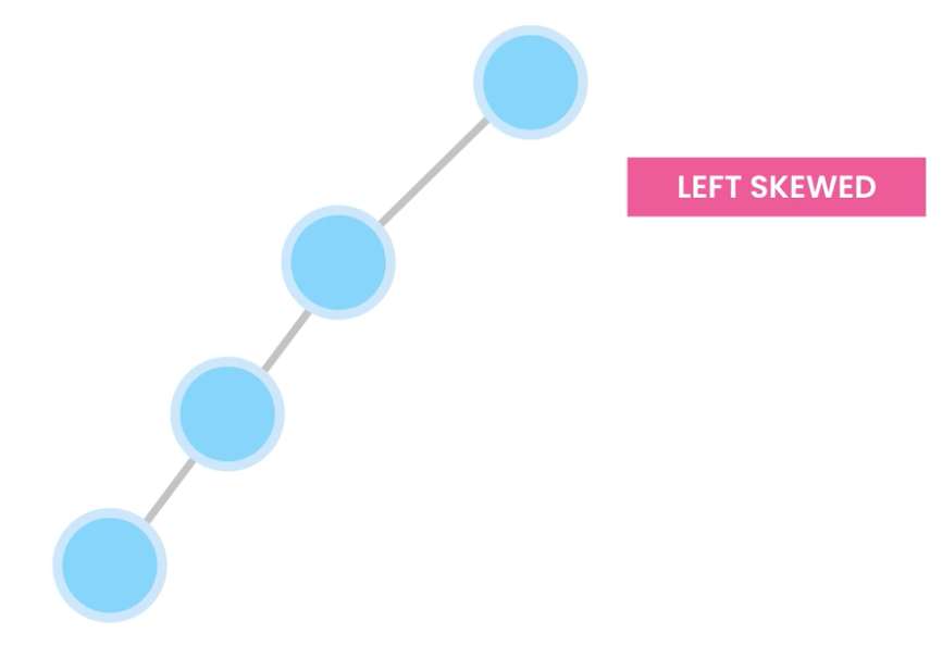
It becomes a linked list and the run time back to O(n).
so…how should we add to BST so that it is more balanced?
AVL (Adelson-Velsky and Landis) is a special BST where it has self-balancing properties. There are other popular trees that also self-balances, such as red-black trees, 2-3 trees, b-trees…etc.
If distance > 1, use rotation to re-balance itself.
4 types of rotation:
Left (LL)
Right(RR)
Left-Right (LR)
Right-Left (RL
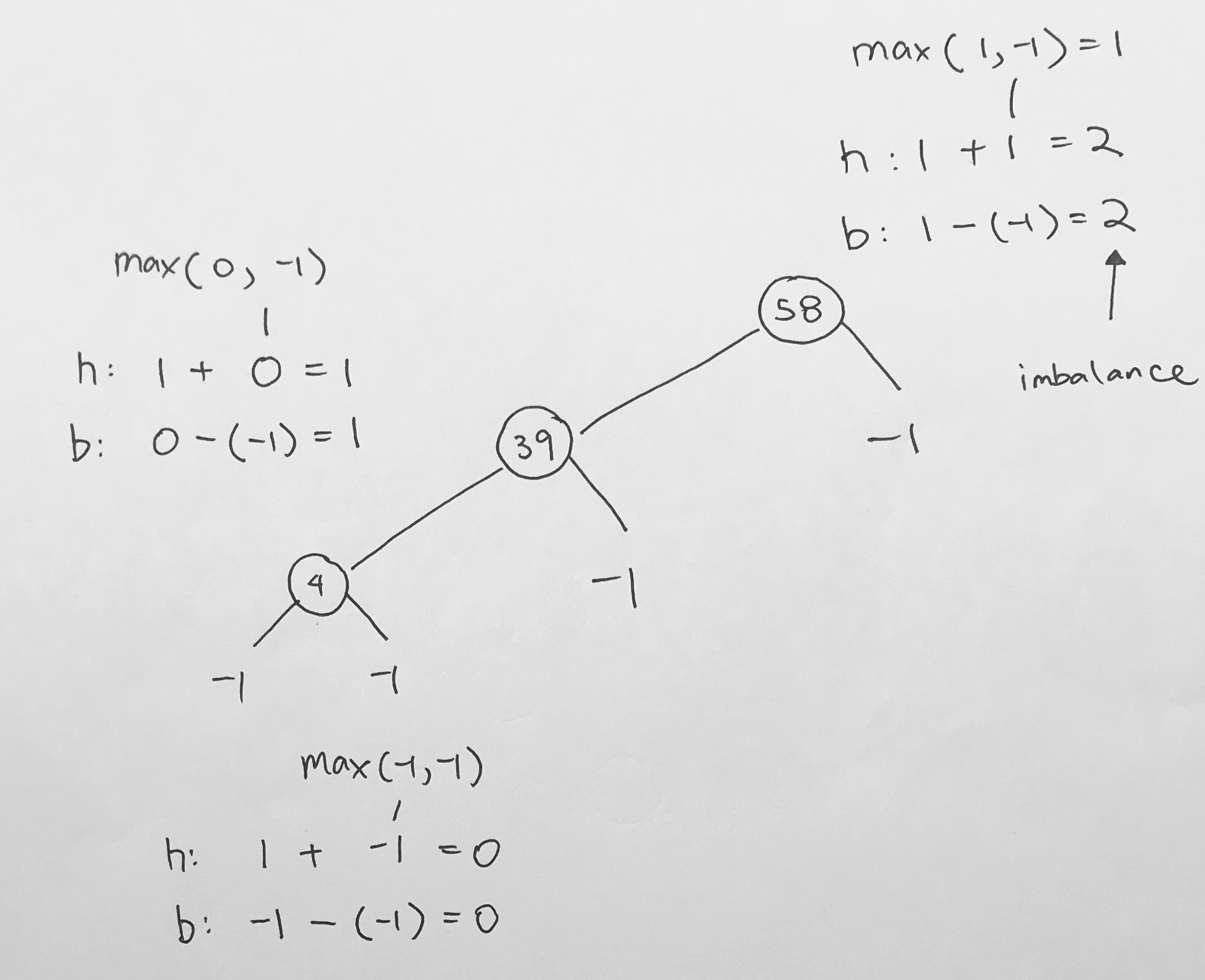
height and balance
The height of a node is the maximum number of vertices from the leaf to itself. Note thath height always start from the ground.
Thus, a leaf has a height of 0.
If the leaf has a parent node, the parent node’s height would be 1.
The balance factor of a node is the height of the left subtree minus the height of the right subtree.
- If the result is > 0, the left subtree is larger
- If the result is < 0, the right subtree is larger
In our example, we use absolute value as we don’t care which side is larger. We simply want to see what the balance factor is.
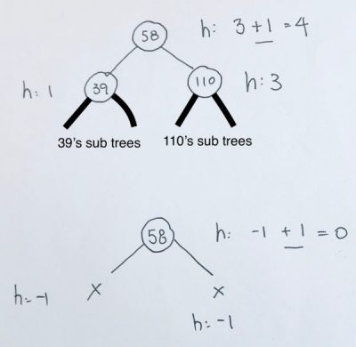
simple example
We have a root node 5, and its left node of value 2.
We calculate from the leaf. 2 is a leaf, so its height is 0. And in turn, balance factor is 0.
The left and right of a leaf is always null, thus, we don’t add 1.
At 5, the height is calculated as height of the subtree + 1. Thus, we get 1 for left subtree. And obviously 0 for right subtree. The height is the max of those 2 numbers. We get 1. The balance is the difference in the height of the left and right subtree, which is 1.
In the next example, it is the same, but simply flipped. The leaf has height of 0 because there is no left or right subtrees. Thus, its balance is also 0.
The root node 8’s left subtree is null, so its height is defaulted to 0.
Its right subtree exists so we add 1 to right subtree height (0), which results to 1.
Our balance is abs value of (left height – right height), which is abs(0-1) = 1.

In the last example, 50 is the root. Its left subtree is 10, which has height of 0, balance of 0.
Its right subtree is 80 which has height of 0, balance of 0.
Thus, at 50, its left height is 0 + 1. right height is 0 + 1, thus, max of left and right height is 1.
Its balance is therefore abs(1 – 1) = 0
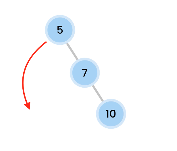
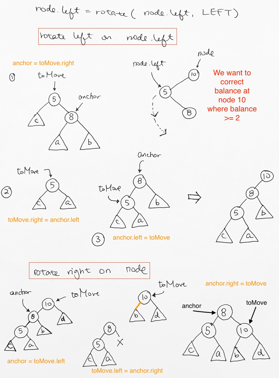
Left Rotation
Right skewed trees are rebalanced by doing a Left Rotation.
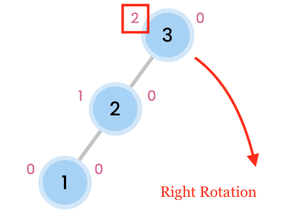
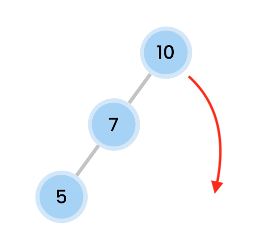
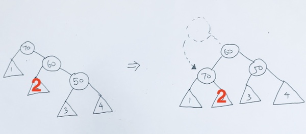
Right Rotation
Left skewed trees are rebalanced by doing a Right Rotation.
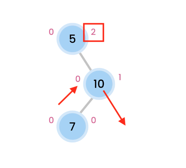
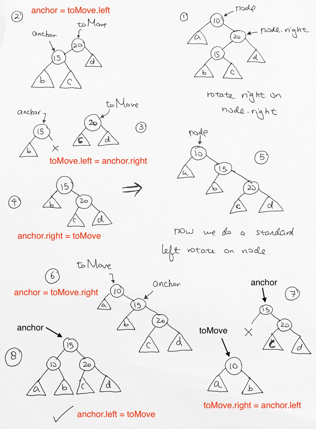
Left Right Rotation
Left rotation on 5, so 7 comes up.
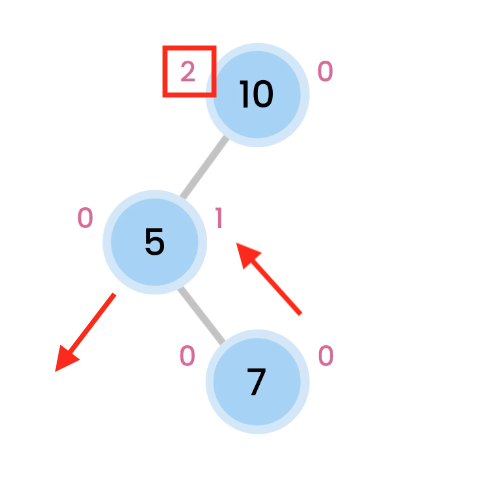
then we do a Right rotation, which makes 10 comes down.
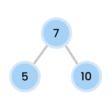
And now, we are balanced.
Left Right Rotation
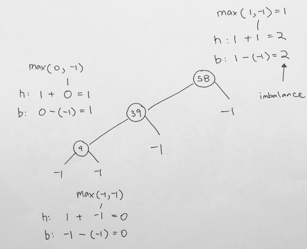
Height Calculations
After inserting new node into an AVL tree, we must re-calculate every node’s height.
|
1 2 3 4 5 |
function heightOfTree(node) { if (node === null) return -1; return Math.max(heightOfTree(node.left), heightOfTree(node.right)) + 1; } |
code for UPDATE of height and balance
The code shows, if we’re at a subtree that is null, we don’t add 1. If there exists a subtree, we add 1 to the height of that subtree in order to get our current height.
We do this for both left and right.
The balance is simply the difference between the heights.
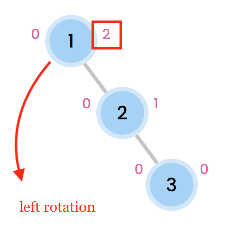
balanceFactor = height(L) – height(R)
> 1 => left heavy, perform right rotation
< -1 right heavy, perform left rotation
|
1 2 3 4 5 6 7 |
// O( 1 ) function calculateAndAssignNewBalance(node) { if (node === null) return 0; let leftHeight = (node.left ? node.left.height: -1); let rightHeight = (node.right ? node.right.height: -1); node.balance = leftHeight - rightHeight; } |
more examples
/ rotation
< rotation
> rotation
\ rotation
In order to fix it, we must do a left rotation.
Insertion with Balance
|
1 2 3 4 5 6 7 8 9 10 11 12 13 14 15 16 17 18 19 20 21 22 23 24 25 26 27 28 29 30 31 32 33 34 35 36 37 38 39 |
// O( log n ) for the insertion function stdBSTInsert(data, node) { // check if reached bottom if (node === null) { return new TreeNode(null, data, 0, 0, null); } // numbers and strings work the same if (data < node.data) { node.left = stdBSTInsert(data, node.left); } else { node.right = stdBSTInsert(data, node.right); } node.height = 1 + Math.max((node.left) ? node.left.height: 0, (node.right) ? node.right.height: 0); // O( 1 ) node.balance = balance(node); // O( 1 ) if (node.balance >= 2) { if (node.left && node.left.balance >= 1) { node = rotate(node, CONSTANTS.RIGHT); // O(log n) } if (node.left && node.left.balance <= -1) { node.left = rotate(node.left, CONSTANTS.LEFT); // O(log n) node = rotate(node, CONSTANTS.RIGHT); // O(log n) } } if (node.balance <= -2) { if (node.right && node.right.balance <= -1) { node = rotate(node, CONSTANTS.LEFT); // O(log n) } if (node.right && node.right.balance >= 1) { node.right = rotate(node.right, CONSTANTS.RIGHT); // O(log n) node = rotate(node, CONSTANTS.LEFT); // O(log n) } } return node; } |
Removal of Node
Removal of Node is straightforward. We use public function remove and it uses utility traverseRemove function. travereRemove traverses the tree until it gets to the node with the value you want to remove.
|
1 2 3 4 5 6 7 8 9 10 11 12 13 14 15 16 |
function traverseRemove(number, node) { if (node == null) { //console.log("Ø You're at leaf end, null. Number " + number + " not found. :P )"); return null; } if (number > node.data) { node.right = traverseRemove(number, node.right); return node; } else if (number < node.data) { node.left = traverseRemove(number, node.left); return node; } else if (number == node.data) { // found what we're looking to delete return node; } } |
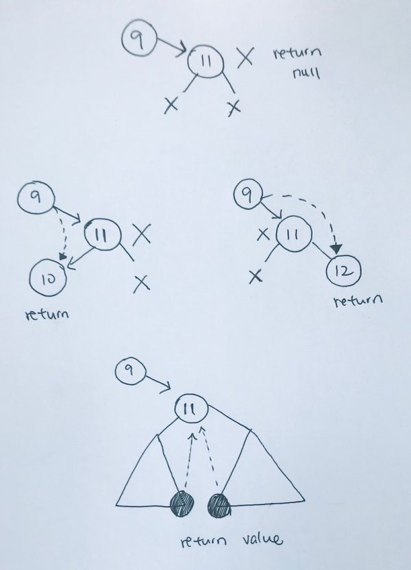
When we find the node we’re looking for, it will look at 4 situations:
1) no children, simply delete and remove the current node
2) only the left child exist, so we return the node’s left subtree to be attached. remove the node
3) only the right child exist, so we return the node’s right subtree to be attached. remove the node.
|
1 2 3 4 5 6 7 8 9 10 11 12 |
if (noChildren(node)) { node.delete(); return null; } if (leftChildOnly(node)) { var leftNodeRef = node.left; node.delete(); return leftNodeRef; } if (rightChildOnly(node)) { var rightNodeRef = node.right; node.delete(); return rightNodeRef; } if (bothChildExist(node)) { // } |
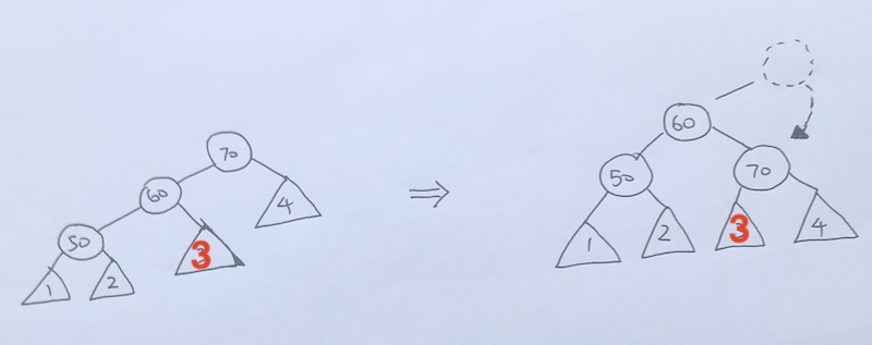
4) both child exist.
This is the key in deletion. In this particular case, we want to return the leftmost of the right subtree or rightmost of the left subtree.
In our example, we return the leftmost of the rightsubtree.
|
1 2 3 4 5 6 7 8 9 10 11 12 13 14 |
function deleteMinimum(node, removeCallBack) { if (noChildren(node)) { removeCallBack(node); return null; } if (rightChildOnly(node)) { removeCallBack(node); return node.right; } if (node.left) { node.left = deleteMinimum(node.left, removeCallBack); return node; } } |
ref – https://github.com/redmacdev1988/avl-binary-tree
Binary Search Tree
http://code.runnable.com/VUTjJDME6nRv_HOe/delete-node-from-bst-for-c%2B%2B
Adding to Tree Concept
Traverse until you hit a leaf. Then, Re-point at the leaf
|
1 2 3 4 5 6 7 8 9 10 11 12 13 14 15 |
//1) we NEED to RE-POINT all left and rights //2) due to 1) we need to carry the tree into the parameter void MyBST::addNode(Node * node, long long newData) { if(newData > node->data) { //right if(node->right) //if the right tree exist, we have to recurse into it this->addNode(node->right, newData); else //if the right tree does not exist, we create a node and point our right to it node->right = new Node(newData); } } |
Finding from Tree Concept
Traverse if data does not match. If at leaf, return NULL.
1) we need the node back, hence, we return our traversals.
2) When we find our target node, we return a new Node with that value. That return will return traverse back.
3) If nothing is found then we return NULL.
|
1 2 3 4 5 6 7 8 9 10 11 12 13 14 15 16 17 18 19 20 21 22 23 24 25 |
//node to traverse into, data to match Node * MyBST::findNode(Node * node, long long newData) { //traverses if(newData > node->data) { //go right if(node->right) { //traverse down return this->findNode(node->right, newData); } else { return NULL; } } //stop case else if (newData == node->data) { cout << "FOUND IT" << endl; return new Node(newData); } return NULL; } |
Running Time
Average Time
Access: O(log(n))
Search: O(log(n))
Insertion: O(log(n))
Deletion: O(log(n))
Worst Time (due to unbalanced tree that deteriorates to a linear tree
Access: O(n)
Search: O(n)
Insertion: O(n)
Deletion: O(n)
The Node – building block of the Binary Search Tree
First we must create the building block of the tree. It is an object with a data container, a left pointer, and right pointer. Each pointer denotes a leaf.
You can initialize this object by value, and set both leafs to NULL.
Or you can pass in data to set everything.
|
1 2 3 4 5 6 7 8 9 10 11 12 13 14 15 16 17 18 19 |
struct Node { int value; Node *left; Node *right; Node(int val) { this->value = val; this->left = NULL; this->right = NULL; } Node(int val, Node * left, Node * right) { this->value = val; this->left = left; this->right = right; } }; |
Creating a BST tree
First we create the BST class. The key thing here is to add a private member for the root Node. This is the starting point of all tree manipulations.
Then we add the void addNode(Node * root, int newVal) for adding data algorithm.
|
1 2 3 4 5 6 7 8 9 10 11 12 13 14 |
class BST { private: Node * root; //head void addNode(Node * root, int newVal); public: BST(); ~BST(); void add(int value); }; |
Adding Nodes O(log n)
We start at the root node, and check the value of it with the incoming new value.
If the new value is larger than the root, then:
1) If the right node exist, we move down the right side of the tree via recursion.
2) If the right node is NULL, we create a new Node, and point it to the right node.
If the new value is smaller or equal than the root, then:
1) If the left node exist, we move down the left side of the tree via recursion.
2) If the left node is NULL, we create a new Node, and point it to the left node.
|
1 2 3 4 5 6 7 8 9 10 11 12 13 14 15 16 17 18 19 20 21 22 23 24 25 26 27 28 |
void BST::addNode(Node * root, int newVal) { GLOG; std::cout << "\n" << __PRETTY_FUNCTION__ << " - value is: " << newVal << std::endl; if(newVal > root->value) { std::cout << "\n" << __PRETTY_FUNCTION__ << " -- newValue is larger than current !! -- "; if(root->right) // new value is larger than current node's value addNode(root->right, newVal); // we go down left else { std::cout << "\n" << __PRETTY_FUNCTION__ << " - Reached end. Creating new Node: (" << newVal << ")" << std::endl; root->right = new Node(newVal); } } else { std::cout << "\n" << __PRETTY_FUNCTION__ << " -- newValue is larger than current !! -- "; if(root->left) addNode(root->left, newVal); else { std::cout << "\n" << __PRETTY_FUNCTION__ << " - Reached end. Creating new Node: (" << newVal << ")" << std::endl; root->left = new Node(newVal); } } } |
http://stackoverflow.com/questions/9456937/when-to-use-preorder-postorder-and-inorder-binary-search-tree-traversal-strate
Depth First Search – Pre order (left side)
print
recursion left
recursion right
If you know you need to explore the roots before inspecting any leaves, you pick pre-order because you will encounter all the roots before all of the leaves.
|
1 2 3 4 5 6 7 8 9 10 |
void BST::traverse(Node * root) { std::cout << "\n" << __PRETTY_FUNCTION__ << " - value is: " << root->value << std::endl; if(root->left) traverse(root->left); if(root->right) traverse(root->right); } |
Depth First Search – Post order (right side)
recursion left
recursion right
print
If you know you need to explore all the leaves before any nodes, you select post-order because you don’t waste any time inspecting roots in search for leaves.
|
1 2 3 4 5 6 7 8 9 10 |
void BST::traverse(Node * root) { if(root->left) traverse(root->left); if(root->right) traverse(root->right); std::cout << "\n" << __PRETTY_FUNCTION__ << " - value is: " << root->value << std::endl; } |
Depth First Search – In order (bottom side)
recursion left
print
recursion right
If you know that the tree has an inherent sequence in the nodes, and you want to flatten the tree back into its original sequence, than an in-order traversal should be used. The tree would be flattened in the same way it was created. A pre-order or post-order traversal might not unwind the tree back into the sequence which was used to create it.
|
1 2 3 4 5 6 7 8 9 10 |
void BST::traverse(Node * root) { if(root->left) traverse(root->left); std::cout << "\n" << __PRETTY_FUNCTION__ << " - value is: " << root->value << std::endl; if(root->right) traverse(root->right); } |
Search for a value O(log n)
Search a value in the binary tree is the fastest. The time is O(log n).
If the node is not NULL, we recursively go down the tree according to if the “to get” value is larger or smaller. Then when we hit a node value that matches, we just return the current node.
|
1 2 3 4 5 6 7 8 |
Node * BST::search(long long value) { if(root) { return this->Traverse(root, value); } else { return NULL; } } |
|
1 2 3 4 5 6 7 8 9 10 11 12 13 14 15 16 17 18 19 20 21 22 23 24 25 26 |
Node * BST::Traverse(Node * root, long long valueToGet) { if(root==NULL) { //std::cout << "Traverse: NULL reached...returning NULL" << std::endl; return NULL; } std::cout << "\n ----STEP----" << std::endl; std::cout << "\n --value to get is: " << valueToGet << std::endl; std::cout << "\n current node's value is: " << root->value; std::cout << "\n-------------------------\n" << std::endl; if (valueToGet < root->value) { return Traverse(root->left, valueToGet); } else if (valueToGet > root->value) { return Traverse(root->right, valueToGet); } else { if(root->value == valueToGet) { //std::cout << "Traverse - value FOUND!" << valueToGet << std::endl; return root; } } return NULL; } |
Deletion O(log n)
Deletion is O(log n + k).
|
1 2 3 4 5 6 7 8 |
void BST::remove(int value) { GLOG; if(root) { this->Delete(root, value); } else { } } |
|
1 2 3 4 5 6 7 8 9 10 11 12 13 14 15 16 17 18 19 20 21 22 23 24 25 26 27 28 29 30 31 32 33 34 35 36 37 38 39 40 41 42 43 44 45 46 |
Node * BST::Delete( Node * root, long long data) { if(root == NULL) return root; //basic traversal else if(data < root->value) root->left = Delete(root->left,data); else if(data > root->value) root->right = Delete(root->right, data); else { //ran to a endpoint or found a node that matches //if no leafs, node without children if(root->left == NULL && root->right == NULL){ delete root; //delete the root root = NULL; } else if (root->left == NULL) { // RIGHT child exists and LEFT is NULL, connect pointer to current's right leaf Node * temp = root; root = root->right; delete temp; } else if (root->right == NULL) { //LEFT child exists and RIGHT is NULL, connect pointer to current's left left Node *temp = root; root = root->left; delete temp; } else { //if BOTH leafs exist, replace the current node's value as the minimum of the right tree Node * rightMin = FindMin(root->right); //find minimum of right tree root->value = rightMin->value; //have current's value take on right tree's minimum root->right = Delete(root->right, rightMin->value); //then search and destroy that value } } return root; } |
Delete All Nodes
The idea behind deleting all the nodes is a thorough recursion through the left and right.
We delete in 2 situations:
1) delete the node if it has no children
2) delete the node after left and right recursion.
given that if a root is NULL, we just return.
If a node has one child (and the other is NULL), then the NULL leaf just returns.
We recurse down the child.
BST.cpp
|
1 2 3 |
BST::~BST() { DeleteAllNodes(root); } |
|
1 2 3 4 5 6 7 8 9 10 11 12 13 14 15 16 17 18 19 20 21 22 23 24 25 26 27 28 29 30 31 32 |
void BST::DeleteAllNodes(Node * root) { //nothing to delete if node is NULL, just return if(root==NULL) { return; } else { //when we reach a node with NO children, we delete it if((root->left==NULL)&&(root->right==NULL)) { cout << "deleting " << root->value << endl; root->value = NULL; root->left = NULL; root->right = NULL; delete root; return; } //when we reach a node with 1 or more child, recurse down DeleteAllNodes(root->left); DeleteAllNodes(root->right); //when both children trees are processed, delete current cout << "deleting " << root->value << endl; root->value = NULL; root->left = NULL; root->right = NULL; delete root; return; } } |
Testing it all
|
1 2 3 4 5 6 7 8 9 10 11 12 13 14 15 16 17 18 19 20 21 22 23 24 25 26 27 28 29 30 31 32 33 34 35 36 37 38 39 40 41 42 43 44 45 46 47 48 49 50 51 52 53 54 55 56 57 58 59 60 61 62 63 64 |
#include <iostream> #include <thread> #include "BST.hpp" #include <random> using namespace std; //Using a BST, 100 million sorted entries takes 30 steps, and 0.00065600s on a 2013 iMac #define TOTAL_NUM 1000000 //http://stackoverflow.com/questions/31015456/is-there-a-way-i-can-get-a-random-number-from-0-1-billion //http://stackoverflow.com/questions/876901/calculating-execution-time-in-c //http://www.bogotobogo.com/cplusplus/multithreaded4_cplusplus11.php void searchFor(long long num, BST * tree) { clock_t tStart = clock(); Node * n = tree->search(num); printf("Time taken to search the tree: %.8fs\n", (double)(clock() - tStart)/CLOCKS_PER_SEC); if(n) { std::cout << "node with data: " << n->value << " found"; } else { std::cout << "\n this tree does not data: " << 888; } } void createUniques(BST * tree) { cout << "----- createOneBillionUniques ---------" << endl; random_device rd; mt19937 gen(rd()); uniform_int_distribution<> dis(1, TOTAL_NUM); //1 billion //1 billion !!! clock_t tStartBuild = clock(); for (int n=0; n<10; ++n) { //cout << "\t index " << n << ", "; tree->add(dis(gen)); } printf("Time taken to build the TREE: %.8fs\n", (double)(clock() - tStartBuild)/CLOCKS_PER_SEC); cout << "\n NODES ADDED \n" << endl; searchFor(8888, tree); delete tree; } int main(int argc, const char * argv[]) { cout << " -------- BST demonstration ------ \n"; BST * myTree = new BST(); thread t1(createUniques, myTree); t1.join(); return 0; } |
merge sort
Typescript
Part 1 – The split
Originally, we recurse into a function, along with a base case.
|
1 2 3 4 5 6 7 8 |
function recursion(index: number) : void { console.log(index); if (index <= 0) { return; } // (1) base case recursion(index-1); // (2) console.log(index); } recursion(3); |
Printing the parameter first will count down from 3.
When we hit our terminating case of zero at (1), we return, and execution from the recursion continues downwards at (2).
As each function pops off from the stack, we log the index again. This time we go 1, 2, and finally back to 3.
Thus display is:
3 2 1 0 1 2 3
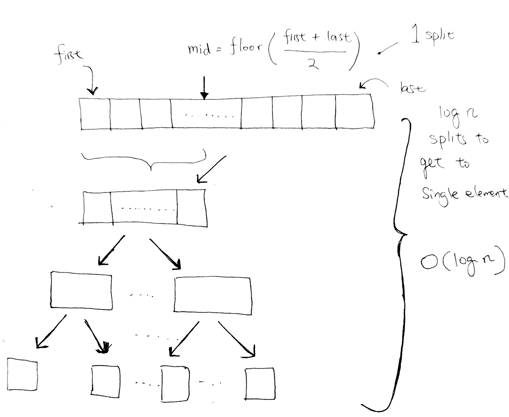
In Mergesort, the idea is that there is a total of n elements. We use splitting in half in order to cut down everything into single elements. Each cut is the same concept behind going down one level in a binary tree. We half all the elements.
In order to reach single elements, the running time is the height of the tree, or (log n) splits.
And in order to go into each halved section to split some more, we use recursion.
Let’s look at how MergeSort does this split:
in code:
|
1 2 3 4 5 6 7 8 9 10 11 12 13 14 15 16 17 18 19 20 21 22 23 24 25 26 27 |
type StrOrNumArr = number [] | string []; class MergeSort { private _data: StrOrNumArr; constructor(arr: StrOrNumArr = null) { this._data = arr ? arr : ["haha", "hoho", "hehe", "hihi", "alloy", "Zoy"]; } private split(start: number, end: number) { if (start >= end) { // Reached single element, stop the recursion console.log(this._data[start]); // print it return; } const mid = Math.floor((start+end)/2); this.split(start, mid); this.split(mid+1, end); } public run() { this.split(0, this._data.length-1); } } const test = new MergeSort(); test.run(); |
The output is:
haha, hoho, hehe, hihi, alloy, Zoy
Part 2 – The Merge
Printing the words out is our first step, and we’ve used recursion. Now we need to compare each word and sort everything.
When we get to haha, we return an array with “haha”. Same with “hoho”. As we recursive back down the stack one step, we now have two arrays. We need to compare everything in these two arrays and sort them into a new array.
- We first create a n space ‘result’ array that is the total length of the arrays.
- We do this so that we will sort each element of these two arrays and put them into our result array.
- We do this until one of the arrays finish.
- Then we just tack on whatever is left from the array that still has untouched elements
|
1 2 3 4 5 6 7 8 9 10 11 12 13 14 15 16 17 18 19 20 21 22 23 24 25 26 27 28 29 30 31 32 33 34 35 36 37 38 39 40 41 42 43 44 45 |
const _left = ["a", "x"]; const _right = ["c", "m", "r", "z"]; function merge(leftArr, rightArr) : StrOrNumArr { let resultIndex = 0; const resultArr = new Array(leftArr.length + rightArr.length); let leftIndex = 0; let rightIndex = 0; while ((leftIndex <= leftArr.length - 1) && (rightIndex <= rightArr.length - 1)) { const leftElement = leftArr[leftIndex]; const rightElement = rightArr[rightIndex]; if (leftElement < rightElement) { resultArr[resultIndex++] = leftElement; leftIndex++; } if (rightElement < leftElement) { resultArr[resultIndex++] = rightElement; rightIndex++; } } // leftover at left array if (leftIndex < leftArr.length) { while (leftIndex < leftArr.length) { resultArr[resultIndex++] = leftArr[leftIndex++]; } } // leftover at left array if (rightIndex < rightArr.length) { while (rightIndex < rightArr.length) { resultArr[resultIndex++] = rightArr[rightIndex++]; } } console.log('result', resultArr); return resultArr; } merge(_left, _right); |
Full code
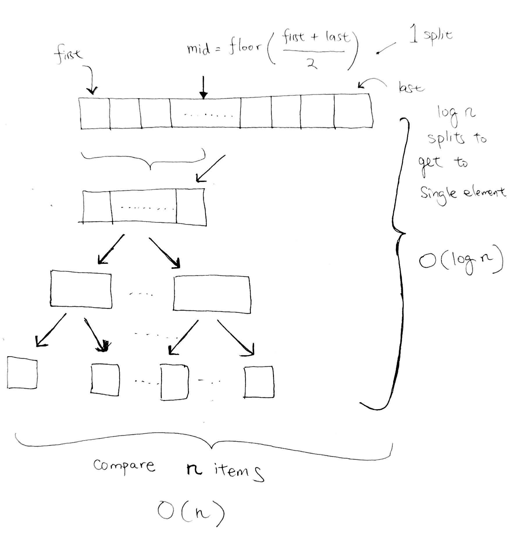
Each level represents one split. And we have a total of (log n) split.
At every level, we do a comparison for every element. Thus our running time for the sort is O(n log n).
The standard merge sort on an array is not an in-place algorithm, since it requires O(N) additional space to perform the merge. During merge, we create a result array in order to carry the left and right array. This is where O(n) additional space comes from:
|
1 |
const resultArr = new Array(leftArr.length + rightArr.length); |
However, there exists variants which offer lower additional space requirement.
It is stable because it keeps the ordering intact from the input array.
Say we have [‘a’, ‘a’, ‘x’, ‘z’]. We split until we get single elements.
[‘a’, ‘a’] and [‘x’, ‘z’]
[‘a’] [‘a’] [‘x’] [‘z’]
We compare ‘a’ and ‘a’.
|
1 2 3 4 5 6 |
if (rightElement === leftElement) { resultArr[resultIndex++] = leftElement; resultArr[resultIndex++] = rightElement; leftIndex++; rightIndex++; } |
This is where it is stable because we always keep the 1st ‘a’ before the 2nd ‘a’ in the results array, which requires O(n) Auxiliary space, during the merge.
We place the leftmost ‘a’ first. Then we put the right side ‘a’ next into the result array.
Say we have another sample data where [‘a’, ‘z’, ‘m’,’b’, ‘a’, ‘c’] and we start recursing via mid splits:
[‘a’, ‘z’, ‘m’] [‘b’, ‘a’, ‘c’]
[‘a’, ‘z’] [‘m’] [‘b’, ‘a’] [‘c’]
[‘a’] [‘z’] [‘m’] [‘b’] [‘a’] [‘c’]
Now we star the merge process:
[‘a’, ‘z’] [‘m’] [‘a’, ‘b’] [‘c’]
[‘a’, ‘m’, ‘z’] [‘a’, ‘b’, ‘c’]
As you can see at this part, we do the final merge and because ‘a’ === ‘a’, we always insert the left-side ‘a’ inside of our results array first. Then we place the right-side ‘a’. Thus, keeping it stable.
Full Source (Typescript)
|
1 2 3 4 5 6 7 8 9 10 11 12 13 14 15 16 17 18 19 20 21 22 23 24 25 26 27 28 29 30 31 32 33 34 35 36 37 38 39 40 41 42 43 44 45 46 47 48 49 50 51 52 53 54 55 56 57 58 59 60 61 62 63 64 65 66 67 68 69 70 71 72 73 74 75 76 77 78 79 80 81 |
type StrOrNumArr = number [] | string []; class MergeSort { private _data: StrOrNumArr; public _chops: number; constructor(arr: StrOrNumArr = null) { this._data = arr ? arr : ["haha", "hoho", "hehe", "hihi", "alloy", "Zoy", "ABC", "you know me", 'michael', 'Jackson']; } // O(n) - linear time to merge private merge(leftArr, rightArr) : StrOrNumArr { let resultIndex = 0; // auxiliary space O(n) const resultArr = new Array(leftArr.length + rightArr.length); let leftIndex = 0; let rightIndex = 0; while ((leftIndex <= leftArr.length - 1) && (rightIndex <= rightArr.length - 1)) { const leftElement = leftArr[leftIndex]; const rightElement = rightArr[rightIndex]; if (leftElement < rightElement) { resultArr[resultIndex++] = leftElement; leftIndex++; } if (rightElement < leftElement) { resultArr[resultIndex++] = rightElement; rightIndex++; } if (rightElement === leftElement) { resultArr[resultIndex++] = leftElement; resultArr[resultIndex++] = rightElement; leftIndex++; rightIndex++; } } // leftover at left array if (leftIndex < leftArr.length) { while (leftIndex < leftArr.length) { resultArr[resultIndex++] = leftArr[leftIndex++]; } } // leftover at left array if (rightIndex < rightArr.length) { while (rightIndex < rightArr.length) { resultArr[resultIndex++] = rightArr[rightIndex++]; } } return resultArr; } private split(start: number, end: number) { if (start >= end) { // base cancel recursion case console.log(this._data[start]); return [this._data[start]]; } const mid = Math.floor((start+end)/2); const leftArr = this.split(start, mid); const rightArr = this.split(mid+1, end); return this.merge(leftArr, rightArr); } public run() { console.log('running MergeSort algorithm'); const result = this.split(0, this._data.length-1); console.log('result', result); } } const test = new MergeSort(); test.run(); |
Javascript version
In-Place: The standard merge sort on an array is not an in-place algorithm, since it requires O(N) additional space to perform the merge. There exists variants which offer lower additional space requirement.
Stable: yes. It keeps the ordering intact from the input array.
http://www.codenlearn.com/2011/10/simple-merge-sort.html
Merge Sort has 2 main parts. The 1st part is the double recursion. The 2nd part is the Merge itself.
1) double recursion
2 recursion calls is executed, one after the other. Usually, in a single recursion, we draw a stack with the recursion and its parameter, and calculate it that way.
However, with two recursions, we simply have more content on the stack in our drawing.
For example, say we have an array of integers, with index 0 to 10.
mergeSort says:
|
1 2 3 4 5 6 7 8 9 10 11 12 13 14 15 |
private void mergeSort(int[] array, int left, int right) { if (left < right) { //split the array into 2 int center = (left + right) / 2; //sort the left and right array mergeSort(array, left, center); mergeSort(array, center + 1, right); //merge the result merge(array, left, center + 1, right); } } |
So we call mergeSort recursively twice, with different parameters. The way to cleanly calculate them is to
write out the parameters, see if the left < right condition holds. If it does, then write result for the 'center' variable.
Evaluate the 2 mergeSort calls and the merge Call. You will then clearly see the order of execution:
Let’s take a look at how the cursive call operates
Say we have [‘a’, ‘b’, ‘c’, ‘d’, ‘e’]
So we first operate on partition(0, 4).
start = 0, end = 4
[‘a’, ‘b’, ‘c’, ‘d’, ‘e’]
We try to find the floor mid point index:
(0+4)/2 = 2, mid value is ‘c’
Now we have:
partition(0, 2) or partition([‘a’, ‘b’, ‘c’])
partition(3,4) or partition([‘d’, ‘e’])
Let’s work on the first one:
partition([‘a’, ‘b’, ‘c’])
floor mid point is (0+2)/2 = 1 [0, 1] mid value is ‘b’
Now we have:
partition(0, 1) or partition([‘a’, ‘b’])
partition(2,2) or partition([‘c’])
We try to find mid point index:
(0+1)/2 = floor (0.5) = 0
Now we have:
partition(0, 0) or partition([‘a’]) returns ‘a’
partition(1, 1) or partition([‘b’]). returns ‘b’
going up the recursion, partition([‘c’]) returns c.
Great.. so now we have values a, b, c. and finished [‘a’, ‘b’, ‘c’] at the top.
Now we need to process
partition([‘d’, ‘e’])
find mid point index (3+4)/2 = floor(3.5) = 3.
So we get
partition(3,3) returns ‘d’
and partition(4,4) returns ‘e’
|
1 2 3 4 5 6 7 8 9 10 11 12 13 14 15 16 17 18 19 20 21 22 23 24 25 26 27 28 29 30 |
export default class MergeSort { private arr: string []; private start: number = 0; private end: number = 0; constructor(strArr: string []) { this.arr = strArr; this.end = this.arr.length - 1; } private partition(start: number, end: number) { console.log(`start ${start}, end ${end}`) if (start < end) { const floorMid = Math.floor((start+end)/2); console.log(`floorMid - ${floorMid} ${this.arr[floorMid]}`); this.partition(start, floorMid); this.partition(floorMid+1, end); } if (start >= end) { console.log(`[end] - ${start} ${this.arr[start]}`); } } public run() { debugger this.partition(this.start, this.end); } } |
2) The merging itself
The merging itself is quite easy.
- Use a while loop, and compare the elements of both arrays IFF the cur for both arrays have not reached the end.
- Whichever is smaller, goes into the result array.
- Copy over leftover elements from the left array.
- Copy over leftover elements from the right array.
|
1 2 3 4 5 6 7 8 9 10 11 12 13 14 15 16 17 18 19 20 21 22 23 24 25 26 27 28 29 30 31 32 33 34 35 36 37 |
private void merge(int[] array, int leftArrayBegin, int rightArrayBegin, int rightArrayEnd) { int leftArrayEnd = rightArrayBegin - 1; int numElements = rightArrayEnd - leftArrayBegin + 1; int[] resultArray = new int[numElements]; int resultArrayBegin = 0; // Find the smallest element in both these array and add it to the result // array i.e you may have a array of the form [1,5] [2,4] // We need to sort the above as [1,2,4,5] while (leftArrayBegin <= leftArrayEnd && rightArrayBegin <= rightArrayEnd) { if (array[leftArrayBegin] <= array[rightArrayBegin]) { resultArray[resultArrayBegin++] = array[leftArrayBegin++]; } else { resultArray[resultArrayBegin++] = array[rightArrayBegin++]; } } // After the main loop completed we may have few more elements in // left array copy them. while (leftArrayBegin <= leftArrayEnd) { resultArray[resultArrayBegin++] = array[leftArrayBegin++]; } // After the main loop completed we may have few more elements in // right array copy. while (rightArrayBegin <= rightArrayEnd) { resultArray[resultArrayBegin++] = array[rightArrayBegin++]; } // Copy resultArray back to the main array for (int i = numElements - 1; i >= 0; i--, rightArrayEnd--) { array[rightArrayEnd] = resultArray[i]; } } |
Running Time
Running time for the double recursion
Average and Worst time:
O(n log n)
How?
The log n comes from the fact that merge sort is recursive in a binary way.
4 items, takes 2 divisions to get to the base items.
8 items, takes 3 divisions to get to the base items.
…if you keep going like this, you’ll see that its logarithmic in nature.
Running time for the merge
We are dividing the array along the recursive path.
So length n1 and n2 keeps changing and the complexity of merge routine/method at each call.
It is ‘n’ on the first call to recursion (leftArray of size n/2 and rightArray of size n/2)
It is ‘n/2’ on the second call to recursion. (we merge two n/4 arrays)
It is ‘n/4’ on the third call to recursion. (we merge two n/8 arrays)
……. and so on …..
till we merge just 2 items ( leftArray of size 1 and rightArray of size 1) and base case there is just one item, so no need to merge.
As you can see the first call to recursion is the only time the entire array is merged together at each level, a total of ‘n’ operations take place in the merge routine.
Hence that is why its O( n log n )
Binary Array Search
|
1 2 3 4 5 6 7 8 9 10 11 12 13 14 15 16 17 18 19 20 21 22 23 24 25 26 27 28 29 30 31 32 33 34 35 36 37 38 39 40 41 42 43 44 45 46 47 48 49 50 51 52 53 54 55 56 57 58 59 60 61 62 63 64 65 66 67 68 69 70 71 72 73 74 75 76 77 78 79 80 81 82 83 84 85 86 87 88 89 90 91 92 93 94 |
#include <stdio.h> #include <ctime> #include <cstdlib> class OrdArray { private: int * integerArray; int nElems; public: OrdArray(int max) //constructor { nElems = max; integerArray = new int [max]; //srand((unsigned)time(0)); // initialize the RNG for ( int i = 0; i < getSize(); i++) { integerArray[i] = i + 2; } } //parameter is the element that we want to find int find(int elementToFind) //initial find() { printf("\n\nI want to find element: %d in the array", elementToFind); return recFind(elementToFind, 0, nElems-1); } int recFind(int elementToFind, int lowerBound, int upperBound) { if(upperBound < lowerBound) { printf("\n\n ------- DOES NOT EXIST------"); return -1; } printf("\n\n Let's check if element %d is at 'floor middle' of index %d to index %d?", elementToFind, lowerBound, upperBound); int floorMiddleIndex = (lowerBound + upperBound ) / 2; printf("\nThe element at middle floor index %d is: %d", floorMiddleIndex, integerArray[floorMiddleIndex]); int floorMiddleElement = integerArray[floorMiddleIndex]; if(floorMiddleElement == elementToFind) { printf("\n\nYES! FOUND IT!"); return floorMiddleIndex; //found it } else { //if we're looking for is larger than our floor middle element, //then we go to upper half of array if (floorMiddleElement < elementToFind) { printf("\ngoing to search from index %d to index %d", floorMiddleIndex+1, upperBound); return recFind(elementToFind, floorMiddleIndex+1, upperBound); } else { //floorMiddleElement >= elementToFind printf("\ngoing to search from index %d to index %d", lowerBound, floorMiddleElement-1); return recFind(elementToFind, lowerBound, floorMiddleIndex-1); } } return -1; } int getSize() { return nElems; } void display() { printf("\n\n"); for (int i = 0; i < nElems; i++) { printf("\n array element %d: %d", i, *(integerArray+i)); } } }; |
Pre print recursion
ref – http://chineseruleof8.com/code/index.php/2015/11/16/simple-recursion/
|
1 2 3 4 5 6 7 8 9 10 11 12 13 |
void countDown( int n ) { //SOL #1 if(n == 0){ // BASE CASE #2 printf("\n\n ~~~ HAPPY NEW YEARRRRRR! ~~~~ "); //#3 return; //EOL #4 } printf("\n\n %d !", n); // #5 countDown(n-1); //#6 //EOL #7 } |
note: recFunc is a placeholder name for any recursive function name that you are running.
a) we write the push of the function for recFunc( 3 ) onto the main stack
b) We begin for the start of line for recFunc( 3 ) at comment #1
c) We check the base case at comment #2, it is false so we move down to comment #5. Its a print statement so we print n, which is 3.
We need to remember to write 3 in the output as shown on the top right hand side of the image.
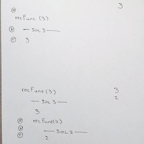
Then we hit comment #6, which is a call to the recursive function. This means we are going to push recRunc( 2 ) onto the stack. Thus:
a) we for visual clarity, we tab some spaces, then write out recFunc( 2 )
b) we reach comment #1 which is the Start Of Line for recFunc( 2 )
c) We check the base case at comment #2, it is false so we move down to comment #5. Its a print statement so we print n, which is 2. Remember to write it in your output section.
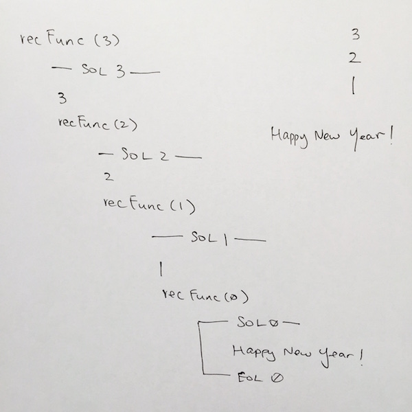
Reaching the base case
We continue this fashion until we hit recFunc( 0 ). Once we get to recFunc( 0 ), we write out SOL at comment #1, then when we reach the base case at comment #2. It evaluates to true, so we print out the “happy new year” at comment #3, and the function returns at comment #4.
Whenever a return or end of function is reached, we pop the stack frame. In our case we pop the stack frame for recFunc( 0 ). On our paper for visual clarity, make sure you draw a line connecting SOL 0 to EOL 0. This tells us that the stack frame for rechFunc has been popped and completed.
In code, we then continue where we left off at comment #6 for recFunc( 1 ). We then go down to comment #7. Its the EOL for recFunc( 1 ), so on our paper, we write out —– EOL 1 —–.
In code, we reach end of function, so that means we pop the stack frame for recFunc( 1 ). Make sure you draw the connecting line from SOL 1 TO EOL 1 to clarify this.
We continue where we left off at comment #6 for recFunc( 2 )…
We keep doing this until all the stack frames have been popped, and we finish running recFunc( 3 ).
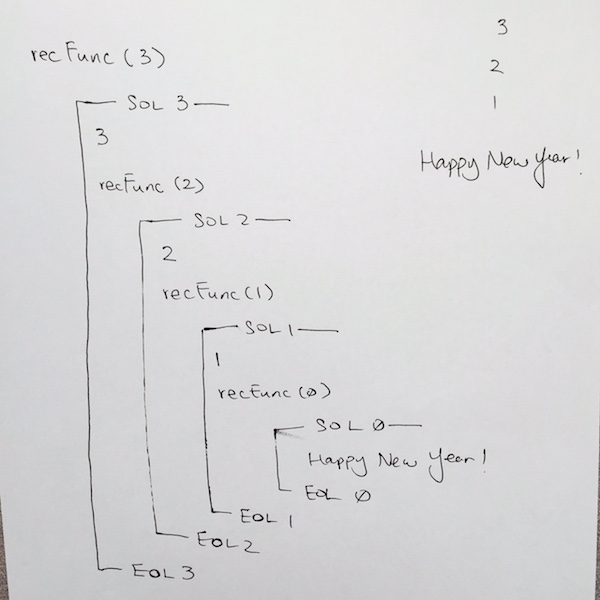
Thus, in the output, you should see: 3 2 1 Happy New Year!
Recursion Concepts
ref – https://www.cs.drexel.edu/~mcs172/Su04/lectures/07.3_recursion_intro/Dangers.html?CurrentSlide=7
https://en.wikipedia.org/wiki/Recursion_termination
Recursion in computer science is a method where the solution to a problem depends on solutions to smaller instances of the same problem. In other words, when a function calls itself from its body.
The power of recursion lies in the possibility of defining an infinite set of objects by a finite statement. In the same manner, an infinite number of computations can be described by a finite recursive program, even if this program contains no explicit repetitions.
A common computer programming tactic is to divide a problem into sub-problems of the same type as the original, solve those sub-problems, and combine the results. This is often referred to as the divide-and-conquer method;
Pros
Less Code – Recursion is generally known as Smart way to Code
Time efficient – If you use recursion with memorization, Its really time saving
For certain problems (such as tree traversal ones) – it’s more intuitive and natural to think of the solution recursively.
Cons
Recursion takes up large amounts of computer resources storing return addresses and states.
In other words, if left unbounded, and fed a data set which leads it deep enough, the function call overhead will accumulate, sucking up system resources rapidly and eventually overflowing the stack.
It is fairly slower than its iterative solution. For each step we make a recursive call to a function, it occupies significant amount of stack memory with each step.
May cause stack-overflow if the recursion goes too deep to solve the problem.
Difficult to debug and trace the values with each step of recursion.
Recursion vs Iteration
Now let’s think about when it is a good idea to use recursion and why. In many cases there will be a choice: many methods can be written either with or without using recursion.
Q: Is the recursive version usually faster?
A: No — it’s usually slower (due to the overhead of maintaining the stack)
Q: Does the recursive version usually use less memory?
A: No — it usually uses more memory (for the stack).
Q: Then why use recursion??
A: Sometimes it is much simpler to write the recursive version (for trees)
- Use recursion for clarity, and (sometimes) for a reduction in the time needed to write and debug code, not for space savings or speed of execution.
- Remember that every recursive method must have a base case (rule #1).
- Also remember that every recursive method must make progress towards its base case (rule #2).
- Sometimes a recursive method has more to do following a recursive call. It gets done only after the recursive call (and all calls it makes) finishes.
- Recursion is often simple and elegant, can be efficient, and tends to be underutilized.
Examples
|
1 2 3 4 5 6 7 8 9 10 11 12 13 14 |
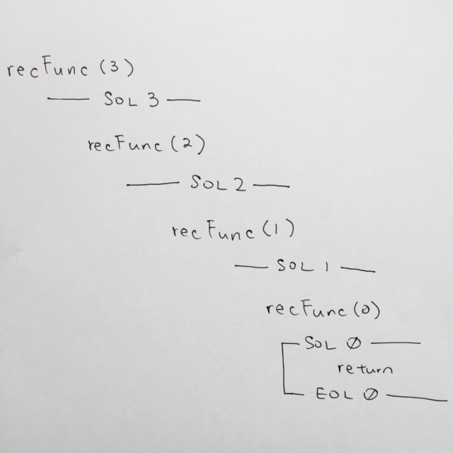
void countDown( int n ) { //n is the counter //SOL Start Of Line #1 //base #2 if(n == 0) { printf("\n\n ~~~ HAPPY NEW YEAR! ~~~~ "); // #3 //EOL #4 return; } countDown(n-1); //recursion #5 //EOL End Of Line #6 } |
Every recursive function has 2 basic parts:
1) A base case return
2) a recursive function.The base case stops the recursion, and the recursive function keeps it running. Our base case would be comment #2. Recursive case would be at comment #5.
In order to properly understand how a simple recursion work, whenever a function is called, on your paper, write out the function name with its parameter. In the pictorial, you will see recFunc(3)
Then on the next line, you want say SOL (start of line). This signifies that you’ve entered the function. In the pictorial, you see —– SOL 3 ——-. Doing this will clarify that you’ve entered the frame for that function.
After the SOL for recFunc(3), we come to base case ( comment #2 ) to see if parameter n is 0.
We see that the base case is not true, so we continue down the code. We come to the recursive case with parameters n – 1 ( comment #5 ). Hence we start a new function stack.
In our paper, we skip a new line and write recFunc(2). This means we’ve entered recFunc( 2 )’s frame ( comment #1 ).
We then do —- SOL 2 —— because we’ve entered the stack for recFunc( 2 ) ( comment #1 ). We then evaluate the base case, to see if parameter n is 0. Its not so we continue on the function call recFunc(1)….
We continue on until we reach recFunc(0).
We see that the base case is true, so we go to comment #3, where you would write out the printf. Then at comment #4, we hit the return for the base case. The return means we pop the stack frame for recFunc( 0 ).
Note: Whenever a stack frame is popped, make sure you connect the lines from SOL to EOL. This can visually help you to see where the function frame has been completed.
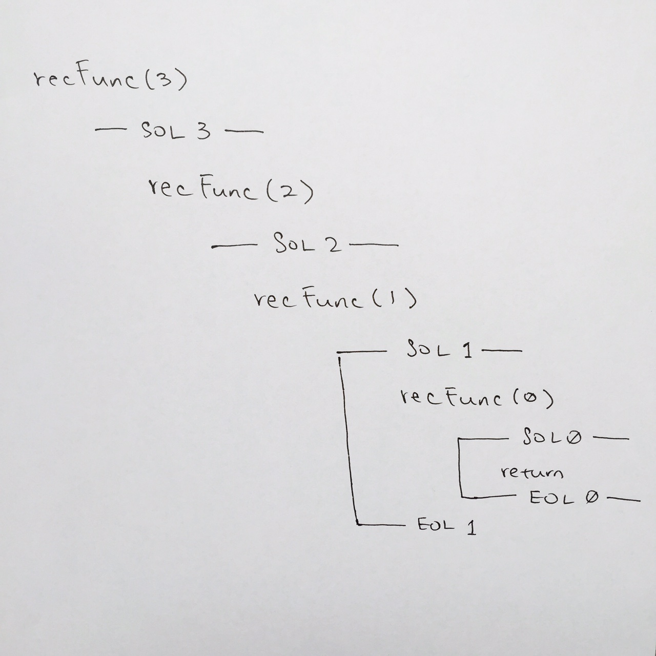
By popping recFunc( 0 ), we continue where we left off at comment #5 of recFunc( 1 ).
We step through the code and hit EOL ( comment #6 ). So in our diagram, we connect the SOL to its EOL to show that we’ve concluded recFunc( 1 ) frame.
We pop the stack for recFunc( 1 ) and we then come to comment #5 for recFunc( 2 ). That is where we left off. We continue down, and we see EOL for recFunc( 2 ) at comment #6. We then draw the end of stack for recFunc( 2 ).
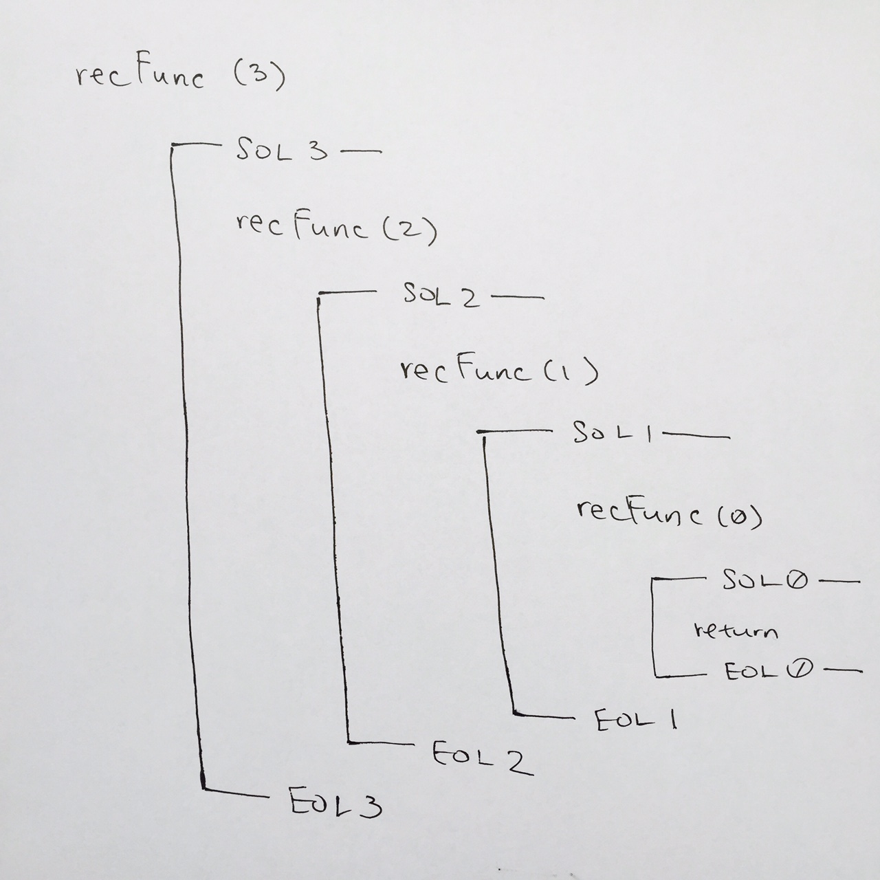
We pop the stack for recFunc(2), and we are then on recFunc(3) at comment #5. We step down, see EOL at comment #6, and in our notes, we draw the end of stack for recFunc( 3 ).
Risks of Recursion
In computing, recursion termination is when certain conditions are met and a recursive algorithm stops calling itself and begins to return values. This happens only if, with every recursive call, the recursive algorithm changes its state and moves toward the base case.
Recursive programs can fail to terminate – This error is the most common among novice programmers. Remember that your subprogram must have code that handles the termination conditions. That is, there must be some way for the subprogram to exit without calling itself again. A more difficult problem is being sure that the termination condition will actually occur.
Stack Overflow – Remember that every subprogram is a separate task that the computer must keep track of. The computer manages a list of tasks that it can maintain, but this list only has a limited amount of space. Should a recursive subprogram require many copies of itself to solve a problem, the computer may not be able to handle that many tasks, causing a system error.
Out of Memory Error – All of the subprograms we have shown here have used pass by value. That means that every time a subprogram is called it must allocate computer memory to copy the values of all the parameter variables. If a recursive subprogram has many parameters, or these parameters are memory intensive, the recursive calls can eat away at the computers memory until there is no more, causing a system error.
Sorted Linked List
download source
The key to understanding sorted insertion is to have 2 pointers.
One is current, the other is trailer.
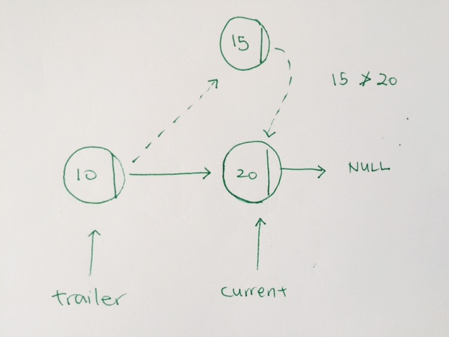
While the current is not NULL, and the incoming data to be inserted is larger than the current’s data, then we move forward
We move forward by having the trailer and current move forward. Trailer take on current. Current take on current’s next.
|
1 2 3 4 5 6 |
while (current != nullptr && data > current->iData) { //traverse forward trailer = current; current = current->pNext; } |
When we do find a node data, where the incoming node’s data is not larger, we stop. We have the trailer’s next point to the new node. The new node’s next take on current.
If the list empty, we simply use the first to point.
|
1 2 3 4 5 |
if(trailer==nullptr) first = new Node(data, first); else //your data is smaller than durrent node data trailer->pNext = new Node(data, current); |