Category Archives: algorithms

algorithms and data structures

Heaps (Binary Tree, priority queues)

code – https://github.com/redmacdev1988/binaryHeap

Another type of Binary tree is the Heap.

A Heap is a binary tree that must have these two properties:

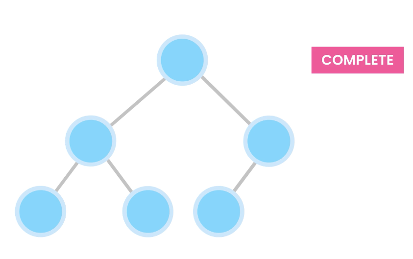
1) A complete binary tree is a binary tree in which every level, except possibly the last, is completely filled, and all nodes are as far left as possible.

Also, nodes are inserted from the left to right.

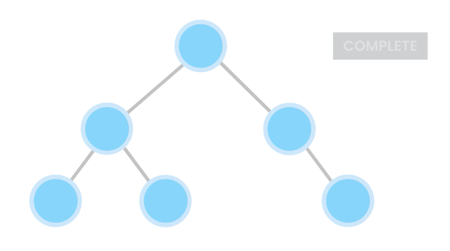
For example, these are complete trees:

Not complete, because because one of the leafs has a hole in it.

2) Heap property – The value of the parent node is greater than or equal to its children.

A heap is a complete binary tree that satisfies the heap property.

When the largest values start from the root, it’s called a max heap.

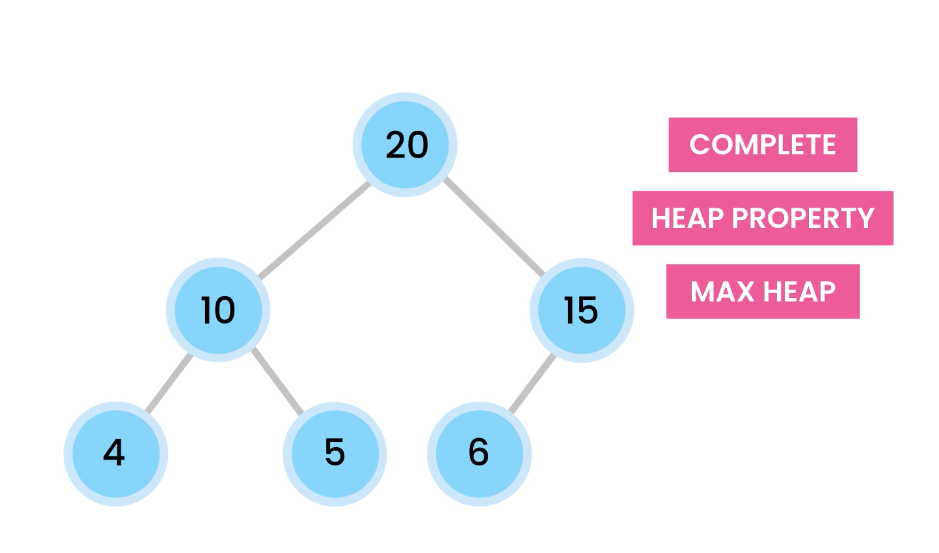
The opposite of that, is the min heap, where the smallest value is at the root.

Applications of Heaps

  • sorting (Heap sort)
  • graph algorithms (Shortest Path)
  • Priority Queues
  • Finding the k-th smallest or largest value

Operations of Heap

[10, 5, 17, 4, 2]

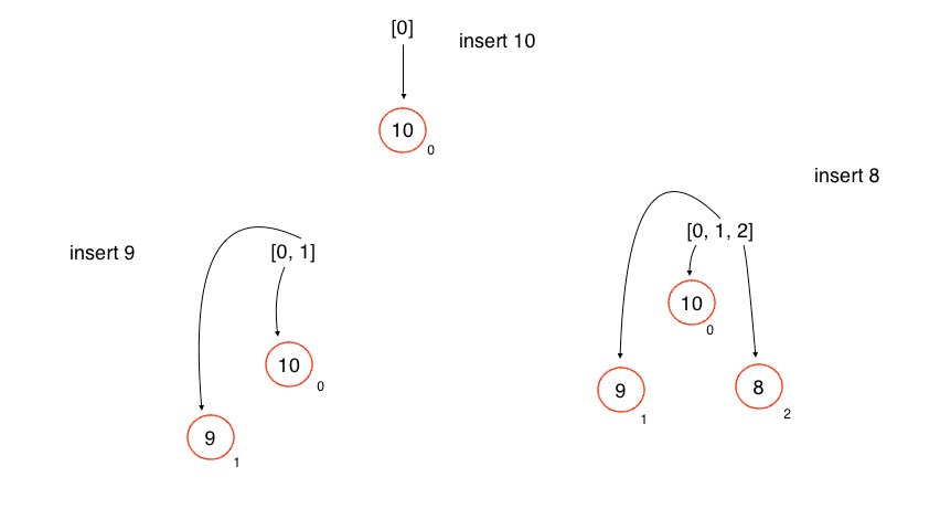
We add 10 the tree as the root.

Then add 5 from the left.

From left to right, we add, so we then add 17.

However, here 17 violates the max heap rule because parents should be larger or equal to children.

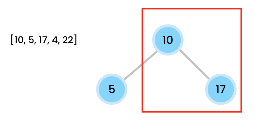
We then bubble the 17. We switch their positions and now 17 is at the root. 5 is on the left. 10 is on the right.

The heap (max heap example)

A max heap has the rule that the parent node must always have a higher priority than its child.

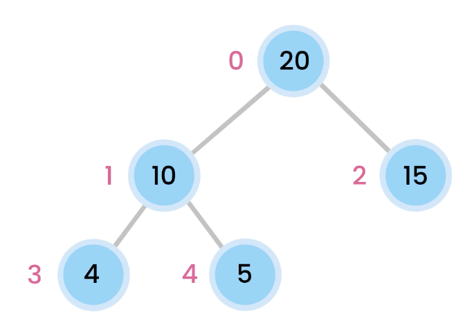
Each node is placed like a tree, however, take caution that there is no left/right references. Everything is accessed via index of the array. If we do want to access children of the node, its children will be indexed like so:

for the left child: 2x + 1
for the right child: 2x + 2

Inserting a node with a larger priority

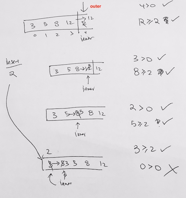
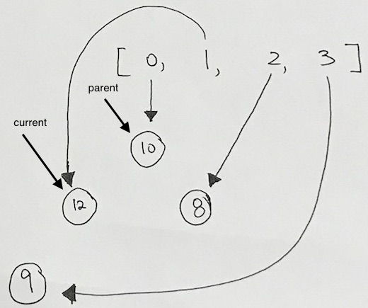
Let’s say we insert a node with a higher priority than its parent. In the example below, we try to insert 12. Obviously, 12 is larger than 8, and thus, we need to readjust.

First, we check to see if its parent (index 1) is valid. It is, so we have the array reference that WAS pointing to the parent, re-point to the the new node.

Then, have the array reference (with index 3) that was originally pointing to the new node, point to the parent.

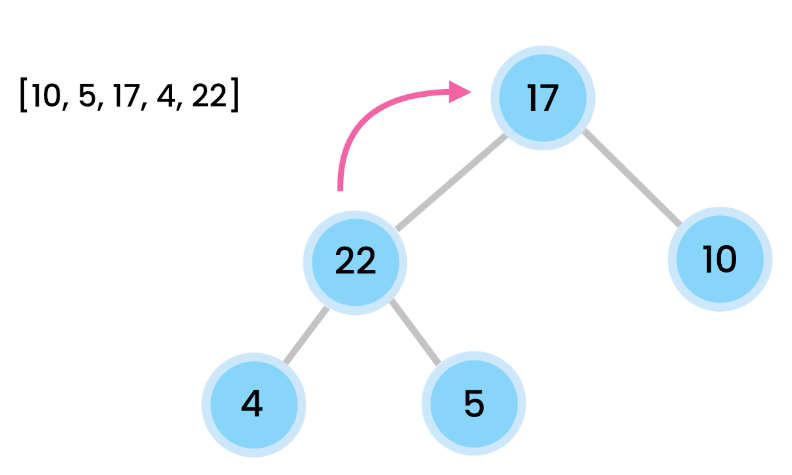
We add 4, it satisfies heap property.

We then add 22. Oops, violation.

Then then swap 22 with 5. And then swap 22 with 17.

When largest values would bubble up.

The longest a value can travel is the height of the tree.
O(log n).

height = log(n).
O(log n).

In heaps, we can only delete the root node. And then fill it in with another value that maintains the heap property.

To do this, we move the last value on the heap (5) to the root. We fix the heap properties by bubbling 5 down and moving 17 up.
We pick larger child and swap.

Time complexity is O(log n) – removing value from heap
Finding max/min value is O(1) – root

Implementation

Store everything in array. Start from root, where index is 0.

left node’s index = parent node index * 2 + 1
right node’s index = parent node index * 2 + 2

index of parent of node = Math.floor((node’s index-1)/2)

Additional Material

We have an array property in the constructor called heap. By definition, this array is contiguous memory, and can be indexed, starting from 0.

When we insert a node to the heap array, we allocate a new Node object in memory. Then the 0th index will contain a reference to that Node. When we insert the next node, another node will be allocated in memory, and we then have the 1st index reference that node.

Every node created will be inserted this way.

Thus, the latest current node will always have index heap.length – 1.

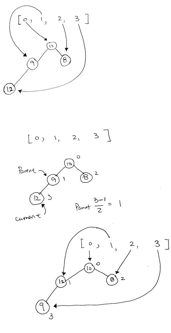
Then we add 12. However 12 violates the heap property.

Now, we recalculate the current node index and the parent node index. We want to move one level up so we can calculate index like so:

The easiest way for us to move up the tree is to simply have the current index take on the parent index. Then, recalculate the parent index via:

Math.floor((currentNodeIdx-1)/2)

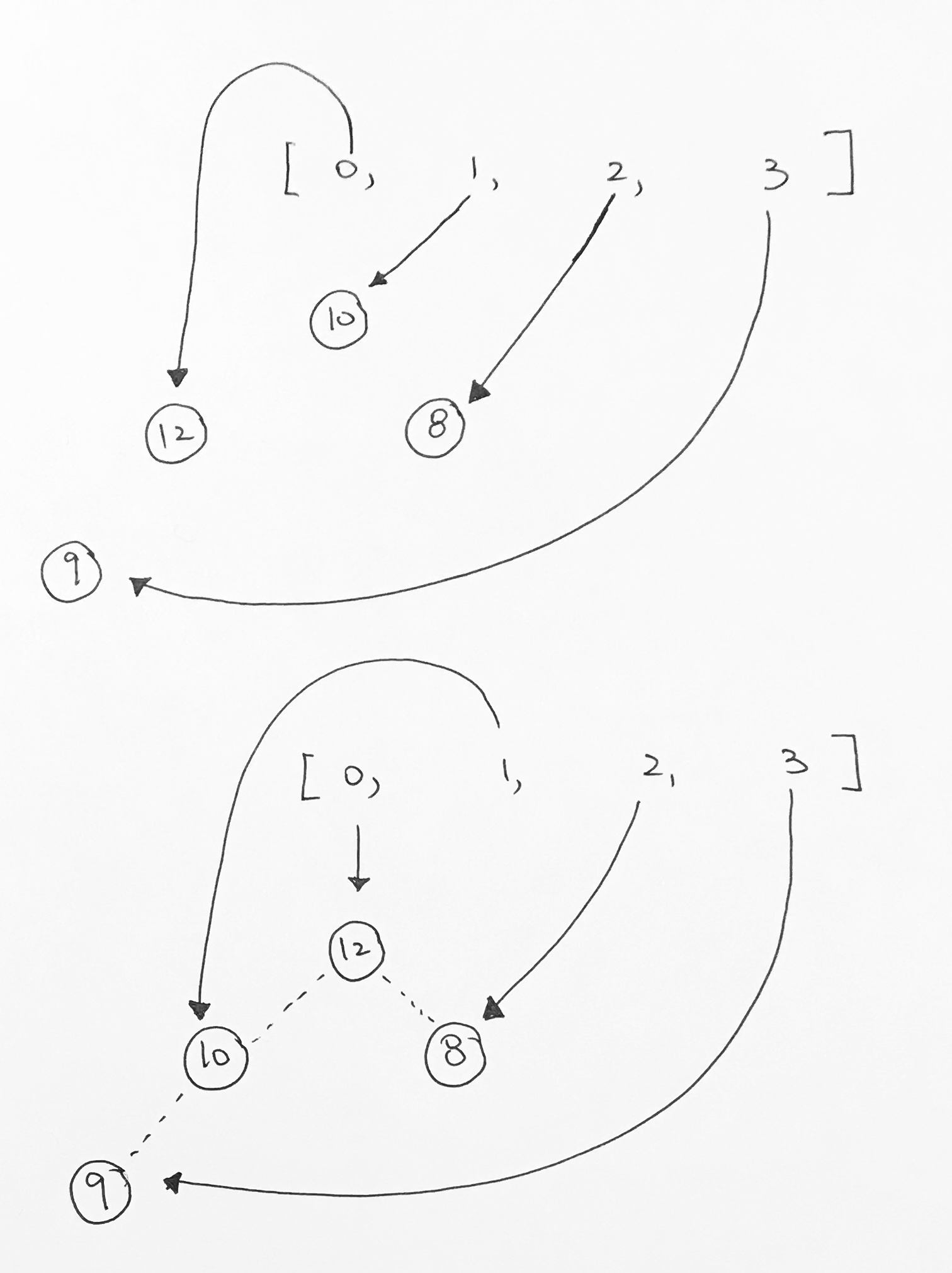
As you see here, we have a violation. 12, being the child of 9, is larger than its parent. So we must bubble 12 up.

After the first bubble, we still have a violation because 12 is larger than its parent 10.
So now we just repeat what we did above.
Is the parent node valid? Yes.
Is the priority of the current node larger than the parent? Yes.

We then have the parent index’s reference point to the larger valued node. And have the current indexed element reference the smaller node. Our nodes gets reshuffled for ease of viewing, but the concept stands. Index 0 is now pointing to the node with the largest value. And all heap properties hold.

insertion code

Note that Math.floor(currentNodeIdx-1/2) is same as Math.ceil(currentNodeIdx-2/2). It gets the parent node’s index.

Heap Removal O( log n )

1) Removal means we pop the root node and process it.
2) Then we get the last element and copy it over to the root node.
3) Use top bottom to push it down if needed.

First, we copy the last value in the tree ( last element of the array ) onto the root. Then remove the last element, and decrease the heap size counter.

From there we recursively push the root value down the tree so that it satisfies the heap property of where key(parent) >= key(child) if its max heap, and <= if its min heap. We decide on which child node to go down by comparing the two child nodes. We switch the parent value with the largest of the 2 child nodes.

Full Source Code

Tests

Heap Sort

[5, 3, 10, 1, 4, 2];

add them into max Heap object.

If we keep popping…they will come out descending order.

if we use min Heap and remove them, it will come out ascending order.

recursive divide and conquer on arrays

Quick sort version

The divide and conquer recursion on an array occurs when we have dubbed a mid,
then recursively go into the left side of the array. Then, the right side. We leave the middle element.

Thus we apply recursion on

  • low to (mid-1)
  • print mid
  • (mid+1) to high

But how?

We recursive into the left

1) For each step we go deeper into the leftmost array, we push one recursion onto the stack. Since we recurse first, then print, we need to push recursions on first.

2) When we reach the 0th element of the array, we have reached the leftmost (single element). Once its reached and the recursion function for the 0th element finishes, we pop it, and then continue on to the next line which is print. In other words, we then start executing the print code after the recursion.

3) When the printing is done (printing the mid), we will hit a function to process the right side.

We recursive into the right

4) Due to the order of the print, and recursion, we have printed, then push a recursion function onto the stack to process the right side.

5) Once that’s done, we pop and then come back to the previous left recursion. We move on and print. Then recurse on the right side.

Let’s go into an example.

Recurse deep into the leftmost array item

Say we have an array with 1 to 9. Indexed from 0 to 8. The concept of recursive divide and conquer is that we calculate a pivot first. The pivot is calculated to be somewhere in the middle of the array, then the left and right array are recursively processed.

For simplification purposes, we want to keep things simple. So let’s calculate the pivot such that it is:
floor of (low + high)/2

low: 0
high: 8

pivot = floor(4) = 4, we’ll print this pivot AFTER we process the left array

Our pivot will be printed after all the left array is processed.

Then we recursively process the left array.

low: 0
high: 3

pivot = floor( 0 + 3 /2 ) = 1, we’ll print this pivot AFTER we process the left array

left array is divAndCon(0, 1-1) or divAndCon(0,0)

It happens that divAndCon(0, 0) is a base case (We notice that low == high) and thus, simply prints 0. We then pop the current recursion function and move on.

Processing the right array

Now we pop back to the previous recursion with indexes divAndCon(0, 3). Since we’ve processed the left array of [1], we need to print the mid, which is index 1, element 2. Then we move on to process the right array [2,3]

right array is divAndConq(2,3)

Notice the array we’re processing is [3,4] where:

low: 2
high: 3
mid = floor of (3 + 2 ) / 2 = 2, we’ll print this pivot AFTER we process the left array

left array is divAndCon(2, 2-1) or divAndCon(2, 1)

When we reach to divAndConq(2,1) we see that low > high is false. Thus, we don’t do anything and just return

Once we return, we need to print the the pivot, which is element 3 at index 2.


Then process the right array, which is divAndCon(2+1,3), divAndConq(3,3)

divAndConq(3,3), we see that low == high, and we print (process)

So as you can see, this is how each element is printed (processed) from the beginning to end in a recursive fashion on an array.

Left Recursion not available

There comes a situation where the start index is larger than the end index…

for example, say we’re at recursion where index is 2 and 3.

[2:X][3:Y]

midpoint = (3 – 2)/2 = 0.

So we go into the LEFT recursion like so divideAndConquer(0, 0-1), or divideAndConquer(0,-1).
Under such case, we do not have a left section to go into. We already have mid pointing to the first element in the current array at [2:X].

Thus, mid will print, and all we have to do is take care of the right element [3:Y] in our right recursion.

Hence, we have to implement a base case to avoid this situation:

whenever start > end, we simply return

Source Code

output

Using divide and conquer to loop

output

MergeSort version

The difference is that the recursion in mergesort does not leave out the mid element. It includes the mid element as part of the right array. Thus, that’s why we use Math.ceil when we divide the array. Thus the recursion is applied on

  • low to (mid – 1)
  • mid to high

We want to drill down to the single element itself, which is when low == high. Then we simply return it. The merge function then proceeds to calculate and sort the returned single elements in 2s. Sorting first, 2 elements. Then the next merge call will sort 4 elements. Then sort 8 sorts, and so on.

where the merge happens like so:

output

Futher study

If you want to reverse the display of the array, simply reverse your recursion like so:

This way, you look at the high end first, which is the upper half. Then the next recursion will go upper half. so on, and so on, until you hit the last element first.

shellsort (js)

Shellsort is the same as insertion sort. Except that it uses a pass array to decide how many number of steps to jump.

In Insertion Sort, we always use 1 step. When we backtrack, we go back 1 step. But in Shellsort, we have an array, where we decide how many jumps to backtrack. This is called a “gap”. Of course in the very end, we’ll definitely have 1 step at the end.

In our example, we decide to use 5, 3, 1. What this means is that we will sort this via Insertion via passes where we jump 5 steps, then 3 steps, then 1 step. So for step 5, we start at index 5 of the array. Do the Insertion sort, but instead of using 1 step when going backwards, we use 5 steps.

first pass, 5 steps

We start off at index 5. Will process the insertion sort, and when we’re done, we go down the array 1 by 1.

The insertion sort itself will use 5 steps when sorting via

Everything else is processed the same way as Insertion Sort. We get the current valueToInsert. It needs to satisfy a few points:

1) is the index larger or equal to the gap index?
2) is the previous gapped element larger than the valueToInsert?

If so, we assign the previous gapped element to the current one.
If not, we just put the valueToInsert back to the current element.

Given the Insertion Code with the gap element like so:

The gap we use is 5. So we need to do an Insertion pass where the gap is 5.

We start index 5. The value at that index is 11. 11 is the value we need to check and find a proper place to insert.

The Insertion sort happens when we have j point to i.

1) j>= gap, 5 >= 5 ? yes
2) previous gapped element > valueToInsert, 6 > 11 ? NO

dataStore[5] = 11, we move down the array.

shellsort_pass5_1

The next index is 6. dataStore[6] is 8. The previous gapped element is dataStore[6-5] is 0

1) j >= gap, 6 >= 5? yes
2) previous gapped element > valueToInsert, 0 > 8, NO

dataStore[6] = 8, we move down the array

shellsort_pass5_2

The next index is 7. dataStore[7] is 0. Its previous gapped element dataStore[7-5] is 2.

1) j >= gap, 7 >= 5? yes
2) previous gapped element > valueToInsert, 2 > 0 yes

When both requirements is true, we exchange the element values. Basically storing the previous value into the current value. This is the because the previous value is larger than the current value.

We continue on the insertion sort by looking back at -gap elements. Namely, j-= gap. Hence our j is now at index 2, dataStore[2] = 2.
We check the requirements again:

1) j >= gap, 2 >= 5 NO

So we jump out of the loop and assign the valueToInsert at dataStore[2]. This perfectly switches the numbers at dataStore[2], and dataStore[7].

shellsort_pass5_3

We move onto the next index at 8. dataStore[8] is 5.
Previous gapped element is dataStore[8-5] = 9

1) j >= gap, 8 >= 5, yes
2) previous gapped element > valueToInsert, 9 > 5 yes

Hence we need to copy the previous element to the current one. We then backtrack gap steps into index 3

1) j >= gap, 3 >= 5, NO
therefore dataStore[3] = 5.

We keep going down the array.

shellsort_pass5_4

We process the last element at index 9, dataStore[9] is 4.

dataStore[9] is 4
dataStore[9-5] is 3

1) j>= gap, 9 >= 5
2) previous gapped element > valueToInsert, 3 > 4, NO.

So we jump out of the loop
dataStore[9] = 4

next gap pass, 3 steps

We start from beginning to end, and at index gap. We do the insertion sort with gap steps, however, we process each element down the array one by one.

index 3

Hence, our next pass involves gap 3. We start off at index 3.
We see that dataStore[3] is 9. valueToInsert = 9.
Previous gap element is dataStore[0] is 6.

is index 3 >= 3 yes
6 > 9 (valeToinsert) NO, move on to next index

shellsort_pass3_1

index 4

We now on index 4.
dataStore[4] = 3, valueToInsert = 3
dataStore[4-3] = 0

4 >= 3 yes
0 > 3 (valeToInsert) NO, move on to next index

index 5

We now on index 5.
dataStore[5] is 11, valueToInsert = 11
dataStore[5-3] is 2

5 >= 3 yes
2 > 11 (valeToInsert), NO, move on to next index

shellsort_pass3_2

index 6

We now on index 6.
dataStore[6] is 8 valueToInsert = 8
dataStore[6-3] is 9.

6 >= 3 yes
9 > 8(valeToInsert), we then copy over the value from the previous element to the current

Thus, dataStore[6] = 9.

We go back 1 gap step so now j is at index 3.
dataStore[3] is 9
dataStore[3-3] is 6

3 >= 3 yes
6 > 8 (valeToInsert), NO, we skip out. have current index j, dataStore[3] = 8 (valueToInsert)

move forward down the array

shellsort_pass3_3

index 7

We are now at index 7.
dataStore[7] is 0. valueToInsert is 0.
dataStore[7-3] is 3

7>=3 yes
3 > 0 yes

Let’s copy previous element to current so now
dataStore[7] is 3.

j moves a “gap” step back to index 4

dataStore[4] is 3
dataStore[1] is 0

4 >= 3, YES
0 > 0 NO

dataStore[4] is 0.

Move forward

shellsort_pass3_4

index 8

dataStore[8] is 5 (valueToInsert)
dataStore[8-3] is 11

8 >= 3 yes
11 > 5 yes

So we need to copy the previous value over to current.

dataStore[8] = 11

Go back 1 “gap” step to index 5

dataStore[5] is 11
dataStore[5-3] is 2

5 >= 3 yes
2 >= 5 (valueToInsert) NO

dataStore[5] = 5

move on…

shellsort_pass3_5

Index 9

Finally, we are index 9.

dataStore[9] is 4 (valueToInsert)
dataStore[9-3] is 8

9 >= 3 yes
8 > 4 yes

so we copy the previous gap element to current
dataStore[9] = 8

we go previous gap element to index 6

dataStore[6] is 8
dataStore[6-3] is 9

6 >= 3, YES
9 >= 4 (valueToInsert), YES

copy the previous gap element to current
dataStore[6] = 9

go back “gap” elements

dataStore[3] is 9
dataStore[0] is 6

3 >= 3, YES
6 > 4 (valueToInsert) YES

copy the previous gap element to current
dataStore[3] = 6

go back “gap” elements

index is now 0
0 >= 3 NO

so dataStore[0] = 4 (valueToInsert)

Done for gap 3 pass

shellsort_pass3_6

Full Source

Insertion Sort

http://www.geeksforgeeks.org/insertion-sort/

Insertion sort is a simple sorting algorithm that works the way we sort playing cards in our hands

Say we’re given a data set, 8 5 3 12 2

Option 1 – previous is larger

We start off the algorithm at index 1.
So we see 5 and store it in a temp variable.

There are 2 conditions we must satisfy:

1) Is the current index > 0 ? (1 > 0 ? yes )
2) Is the previous element is larger than our temp? 8 > 5, yes.

Both satisfies so we copy the previous element (8) to the current location where 5 is.

We move 1 step back and hit index 0.

We evaluate the 2 situations again:

1) 0 > 0, no. We stop.

If we reach index 0, that means we’ve reached the end, and we store 5 there.

We then move on to index 2 and continue processing in the same manner.

Option 2 – previous is smaller

If say we have 3 5 7.

We start off at index 1.
We see 5 and store it in a temp variable.

There are 2 conditions we must satisfy:

1) Is the current index > 0 ? (1 > 0 ? yes )
2) Is the previous element is larger than our temp? 3 > 5, no.

In this case, we don’t do anything move onto the next index 2.

This is the part where if the whole array is sorted, we only execute this comparison and then move on to the next index. Since the previous will always be smaller than the current, we simply stop and move on. Hence, the best case is O(n) because we do execute a comparison at every index once. We do this for every element and then stop.

Insertion sort takes the current number and go backwards to see where to insert it. We do this by comparing the previous element and seeing if its bigger than our valueToInsert. If it’s larger, push it down and we keep going. If it’s smaller, we stop and we insert our number. If we reach the end at index 0, we insert our number.

insertionsort_ex_a

Now we have 5 8 3 12 2.

We work our next pass which is index 2 with value 3.

We store 3 and start searching for the insertion point. We evaluate the 2 points:

1) is index > 0? 2 > 0, yes.
2) We look at the previous element 8. is 8 > 3? yes, so we move 8 to where 3 is.

Move backwards 1 step.

1) is index > 0? 1 > 0, yes.
2) Then we look at previous element 5, is 5 > 3? yes. so we move 5 to where 8 is.

1) is index > 0? 0 > 0, no. We’ve reached the end. Hence we put 3 at index 0.

This leaves us with 3 5 8 12 2.

insertionsort_ex_b

Then we work on value 12.

1) is index > 0? index 3 > 0, yes.
2) Previous element 8 > 12?
no. We stop, and move on.

Moving on…finally, our last value is 2. Apply the same as we did above and we’ll see that 2 will be inserted at the way in the beginning because it is smaller than the other numbers.

insertionsort_ex_c

full source

Time Complexity

The best case input is an array that is already sorted. In this case insertion sort has a linear running time (i.e., O(n)). During each iteration, the first remaining element of the input is only compared with the right-most element of the sorted subsection of the array.

The simplest worst case input is an array sorted in reverse order. The set of all worst case inputs consists of all arrays where each element is the smallest or second-smallest of the elements before it. In these cases every iteration of the inner loop will scan and shift the entire sorted subsection of the array before inserting the next element. This gives insertion sort a quadratic running time O(n^2).

The average case is also quadratic, which makes insertion sort impractical for sorting large arrays.

However, insertion sort is one of the fastest algorithms for sorting very small arrays, even faster than quicksort; indeed, good quicksort implementations use insertion sort for arrays smaller than a certain threshold, also when arising as subproblems; the exact threshold must be determined experimentally and depends on the machine, but is commonly around ten.

Selection sort

https://en.wikipedia.org/wiki/Selection_sort

Worst-case performance О(n2) comparisons, О(n) swaps
Best-case performance О(n2) comparisons, О(n) swaps

The idea is that we latch onto the first element and deem it being the minimum.
We then go through the rest of the array, and look for anything that is smaller. If so, we swap. This is 1 pass.

At this point, after the 1st pass, we deem first element as minimum. Then we move on
to the next element and call it the minimum. We do another pass and look in the leftover array
to see if there’s anything smaller than our minimum. If so, swap.

We keep doing this, pulling minimum numbers from the array and pushing it towards the front, until
all the elements are sorted from smallest to largest.

selectionsort-outer-inner

So there’s 2 loops: outer and inner.

Outer simply goes through the array.

The inner goes through the remaining elements AFTER the outer via a loop and compares it to the outer.

if the inner element is smaller than the outer element, then we swap. Essentially what is happening is that we are bringing in the smallest element to the front.

Example

Given an array, we make passes on it where:

– we select the starting value to be the minimum.
– we then make (length of array – 1) passes over it. (through all of our passes, the last element will be automatically sorted, so no need to do anything on it)
– For every pass, we need to do the very important action of pulling the minimum from the array and swapping it with the first value.

Example

…continuing on in the same fashion…

Eventually all the smallest number will be swapped to the front, resulting in the list being sorted.

full source

Bubble Sort

http://www.geeksforgeeks.org/bubble-sort/

“Bubble” up the largest number in the array. Once that’s done, we “Bubble” again to the array-1 for the next largest number. We keep doing it until we have “Bubbled” every number in the array.

Think of it as looping through the array and looking at each tuple. If a tuple is where element1 > element2, then we swap. This way, the largest element of this run will “Bubble” up to the end. (very right side).

Due to us checking every tuple, we need to makes sure we check from 1..length-1 and NOT 1..length:

(5 1) 4 2 8 –> [1 5] 4 2 8, Here, algorithm compares the first two elements, and swaps since 5 > 1.
1 (5 4) 2 8 –> 1 [4 5] 2 8, Swap since 5 > 4
1 4 (5 2) 8 –> 1 4 [2 5] 8, Swap since 5 > 2
1 4 2 (5 8) –> 1 4 2 [5 8], Now, since these elements are already in order (8 > 5), algorithm does not swap them.

As tuples, the last index should be
element[last-1], element[last]

Therefore, we only need to check from (index 0) to (< lastIndex-1) because it does not make sense at all to swap the very last element of the array to its next element because the next element does not exist. The last swap we do should be data[lastIndex-1], data[lastIndex]. That is why we give outer - 1 into bubbleUpLargest.

Example

Example:
First Pass:
( 5 1 4 2 8 ) –> ( 1 5 4 2 8 ), Here, algorithm compares the first two elements, and swaps since 5 > 1.
( 1 5 4 2 8 ) –> ( 1 4 5 2 8 ), Swap since 5 > 4
( 1 4 5 2 8 ) –> ( 1 4 2 5 8 ), Swap since 5 > 2
( 1 4 2 5 8 ) –> ( 1 4 2 5 8 ), Now, since these elements are already in order (8 > 5), algorithm does not swap them.

Second Pass:
( 1 4 2 5 8 ) –> ( 1 4 2 5 8 )
( 1 4 2 5 8 ) –> ( 1 2 4 5 8 ), Swap since 4 > 2
( 1 2 4 5 8 ) –> ( 1 2 4 5 8 )
( 1 2 4 5 8 ) –> ( 1 2 4 5 8 )
Now, the array is already sorted, but our algorithm does not know if it is completed. The algorithm needs one whole pass without any swap to know it is sorted.

Third Pass:
( 1 2 4 5 8 ) –> ( 1 2 4 5 8 )
( 1 2 4 5 8 ) –> ( 1 2 4 5 8 )
( 1 2 4 5 8 ) –> ( 1 2 4 5 8 )
( 1 2 4 5 8 ) –> ( 1 2 4 5 8 )

Numerical example

Given: 6 8 0 7 6 4 3 1 5 10

We compare tuples, so we loop a total of length – 1 times.

[6 8] 0 7 6 4 3 1 5 10

is 6 > 8? no

6 [8 0] 7 6 4 3 1 5 10

is 8 > 0? yes, swap

6 0 [8 7] 6 4 3 1 5 10

is 8 > 7? yes, swap

6 0 7 [8 6] 4 3 1 5 10

is 8 > 6? yes, swap

6 0 7 6 [8 4] 3 1 5 10

is 8 > 4? yes, swap

6 0 7 6 4 [8, 3] 1 5 10

is 8 > 3? yes, swap

6 0 7 6 4 3 [8, 1] 5 10

is 8 > 1? yes, swap

6 0 7 6 4 3 1 [8, 5] 10

is 8 > 5? yes, swap

6 0 7 6 4 3 1 5 [8 10]

is 8 > 10? no

pass 1 finished, so as you can see 8 “bubbles up”, until it meets 10.

Since we’re done, we are confident that the last number is largest. 10 is done, so we move our lastIndex down and process the leftover array for the 2nd pass.

[6 0] 7 6 4 3 1 5 8 (10)

is 6 > 0? yes, swap

0 [6 7] 6 4 3 1 5 8

is 6 > 7? no, move on

0 6 [7 6] 4 3 1 5 8

is 7 > 6? yes, swap

0 6 6 [7 4] 3 1 5 8

is 7 > 4? yes, swap

0 6 6 4 [7 3] 1 5 8

is 7 > 3? yes, swap

0 6 6 4 3 [7 1] 5 8

is 7 > 1? yes, swap

0 6 6 4 3 1 [7 5] 8

is 7 > 5? yes, swap

0 6 6 4 3 1 5 [7 8]

is 7 > 8? no

pass 2 finished, so as you can see, 7 “bubbles up”.

0 6 6 4 3 1 5 7 (8) (10) so now, 8, 10 done. We need to process 0 6 6 4 3 1 5 7.

We move our lastIndex down and process the leftover array for the 3rd pass.

..this keeps going until all numbers are sorted from smallest to largest.

the bubble sort

bubbleUpLargest

Then in here, we simply go through all the elements and do its swapping. Think of it as
looping through tuples and swapping them.

The swap function is just a standard swap

Worst-case performance O(n^2)
Best-case performance O(n)
Average performance O(n^2)

The only significant advantage that bubble sort has over most other implementations, even quicksort, but not insertion sort, is that the ability to detect that the list is sorted efficiently is built into the algorithm. When the list is already sorted (best-case), the complexity of bubble sort is only O(n). By contrast, most other algorithms, even those with better average-case complexity, perform their entire sorting process on the set and thus are more complex.

However, not only does insertion sort have this mechanism too, but it also performs better on a list that is substantially sorted (having a small number of inversions).

Bubble sort should be avoided in the case of large collections. It will not be efficient in the case of a reverse-ordered collection.

source code

Hash Table, prime numbers, and hash functions

basic hash table to Strings (xcode 8.3.3)
Hash table with a stack or queue (xcode 8.3.3)
HashTable with choice for data structure

http://www.partow.net/programming/hashfunctions/
https://www.quora.com/Why-are-prime-numbers-used-for-constructing-hash-functions
http://algs4.cs.princeton.edu/34hash/
Why do hash functions use prime numbers?
https://cs.stackexchange.com/questions/11029/why-is-it-best-to-use-a-prime-number-as-a-mod-in-a-hashing-function

Why do hash functions use prime numbers for number of buckets ?

Consider a hash function (or a set of numeric data) that gives you multiples of 10.

If we use a bucket size of say, 4 buckets, we get:

10 mod 4 = 2

20 mod 4 = 0

30 mod 4 = 2

40 mod 4 = 0

50 mod 4 = 2

So from the set of hash results such as {10, 20, 30, 40, 50}, if we were to hash them into our buckets, all of them would go either into bucket 0, or bucket 2. all odd numbers would collide at bucket 2. All even numbers collide at bucket 0. The distribution of data into buckets is not good.

Let’s say we used 7 buckets instead. We take the generated hash keys, and do the mod to see how they are distributed throughout the hash table:

10 mod 7 = 3

20 mod 7 = 6

30 mod 7 = 2

40 mod 7 = 4

50 mod 7 = 1

much better. The numbers are getting distributed more evenly.

Let’s say we used 5 buckets.

10 mod 5 = 0

20 mod 5 = 0

30 mod 5 = 0

40 mod 5 = 0

50 mod 5 = 0

Even though 5 is a prime number, all of our keys are multiples of 5, and thus the mod will always be 0. This will distribute all of our keys into bucket 0.

Therefore, this means we have to choose a prime number that doesn’t divide our keys, choosing a large prime number is usually enough.

the reason prime numbers are used is to neutralize the effect of patterns in the keys in the distribution of collisions of a hash function.

In other words, say we have a function that generates a set (or just a simple data list) of data K

Function generateList generates array: {0, 2, 3, 5, 6, 7, 9, 11, 12, 13, 14, 15, 18, 19, 24, 27, 28, 29, 30, 36, 42, 48 ….etc}

We use a hash table where the number of buckets is m = 12 (non-prime)

Let’s call each number inside of data K, a hash key. So 0 is a hash key. 1 is a hash key. 2 is a hash key. 5 is a hash key, and so on.

We map a hash key onto the bucket size m via AND 0xff, or % array size m. (In our example, we use % array size)

hash-to-bucket
0 % 12 = 0
12 % 12 = 0
24 % 12 = 0
36 % 12 = 0

Thus, for every integer K in our list , 12, 24, 36…would all hash to bucket 0.

The other integers will have their respective buckets
2 % 12 = 2
3 % 12 = 3


13 % 12 = 1
14 % 12 = 2
15 % 12 = 3
18 % 12 = 6
19 % 12 = 7

Given, N is the number of buckets in a hash table. Let’s say 4.

If K is uniformly distributed, in other words, if K has integers (distribution) which has all outcomes equally likely, then the choice of bucket size ‘m’ is not so critical. For example, 1,2,3,4,5,6….etc, thus, K’s integer distribution all comes out equally likely.

However, there is an issue which can arise if the keys being hashed are not uniformly distributed. Specifically when the keys result in values in which N is a factor of that key, or the key is a multiple factor of N.

i.e.

4 is a factor of 20, 40, 60, 80. In the same way, 20 is a multiple factor of 4. 40 is a multiple factor of 4, and so on.

if K is 4, then K is a factor of N (4). 4 % 4 = 0
if K is 20, then K is a multiple factor of N(4). 20 % 4 = 0

4 is factor of 20, 20 % 4 = 0, key 20 get bucket 0
4 is factor of 40, 40 % 4 = 0, key 40 get bucket 0
4 is factor of 60, 60 % 4 = 0, key 60 get bucket 0
4 is factor of 80, 80 % 4 = 0, key 80 get bucket 0

In this situation, integer K, that aren’t factors of N or multiples of factors of N will remain empty, causing the load factor of the other buckets to increase disproportionately.

This situation seems to be the only valid reason to use a prime number. Given that a prime number has only itself and one as factors, using a prime number to resolve this problem means even if the keys are not uniformly distributed and instead possess some of kind structure (specifically multiples of a value), the likelihood that those values will arbitrarily hash to either the value one or N (the prime number) will be vanishingly small.

But, what happens if K is not uniformly distributed? Imagine that the keys that are most likely to occur are the multiples of 10 (like our example above) such as 10, 20, 30, 40, 50…and they keep appearing a lot.

In this case, all of the buckets that are NOT multiples of 10 will be empty with high probability (which is really bad in terms of hash table performance).

In general:

Every key in K (every integer in our array) that shares a common factor with the (number of buckets) m will be hashed to a bucket that is a multiple of this factor.

Every key in K, let’s say 14, which has factors 2, 7.
# of buckets (12) – 2, 3, 4, 6.

14 shares a common factor of 2 with (m, 12 buckets)
Hence any multiples of 14 will be hashed to a bucket that is a multiple of 2.

14 % 12 = 2
28 % 12 = 4
42 % 12 = 6
56 % 12 = 8
70 % 12 = 10
84 % 12 = 0
98 % 12 = 2


Hence, every key in K – 14, 28, 42, 56, …etc
that shares a common factor with (m number of buckets, 12) – common factor is 2
will be hashed to a bucket that is a multiple of that common factor (which is 2, 4, 6, 8)

Therefore, to minimize collisions, it is important to reduce the number of common factors between m and the elements of K. How can this be achieved?

By choosing m to be a number that has very few factors: a prime number.

extending String

initially getting an index from String is used like this:

We call String’s index, use its variable startIndex (which is a static String.Index)
to indicate we start at beginning of the String. Then we off set by i. And that’s where we’ll
return the character in the String.

By using the subscript above, we simply use it to initialize a String, then return that String

Finally, in we extend Character, and create a var ASCII.
In it, we first create a String with its self Character. We access unicodeScalars, which is a
list of ASCII numbers for each character.

Doubly Linked List

xCode demo

Tests

.hpp

.cpp file

Height of Tree

Height of tree is used to find the maximum number of steps to search for an item in a data set using logarithmic division.

If you wanted to find a number in that tree, you compare the toFind integer with the current node. If larger, go down right side. If smaller, go down left side.

You may find your integer at the very top, or at the next node, or a few steps down the tree. But the absolute maximum number of steps it takes to find your item is the height of the tree.

By going down 1 step, you’ve removed half of the data set by process of elimination. For example, if you search for a 2, and the node is 8, you go down the left side. You don’t need to worry about the right side of 8, because all those numbers is guaranteed to be bigger.

With each step you take, you eliminate half of the data set until you finally get to your number.

The number of eliminations (or divisions) you make is basically the height of the tree.

1) get the height of the tree
2) Go through each level of the height and print

level is how many depths to go into the tree..
0 is root
1 means go down 1 level..display all nodes there.
2 means go down 2 levels…display all nodes there..
etc
NOTICE LEVEL. we recursively traverse via LEVEL

QuickSort

http://www.algolist.net/Algorithms/Sorting/Quicksort