Category Archives: algorithms

algorithms and data structures

Algorithm to add a number to every element in an array

June 27, 2021algorithmsadmin

https://www.hackerrank.com/challenges/crush/forum/comments/255515
https://www.hackerrank.com/challenges/crush/forum
https://www.hackerrank.com/challenges/crush/problem

Problem

Given an array of ten elements [0,0,0,0,0,0,0,0,0,0].

Let’s say we are to apply an update to a certain range of indexes…say from a (index 2) to b (index 6), we want to add k (10) to all elements.

[0,0,0+10,0+10,0+10,0+10,0+10,0,0,0]

Let’s denote iteration from a to b as m, this would be O(m) time.
If we were to apply n updates, then we’d end up n * O(m) or O(m*n)
If m or n is huge, then we’d have a performance problem, as it could get close to O(n^2).

How to Solve

So the thing we’re trying to do is to figure out how to express the idea that we want to add a number k from a to b in better running time. Our tactic involves two steps:

1) Assign indices O(x)
2) Calculate sum O(y)

Total running time is O(x+y)

Step One

Use +k and -k at indexes to denote the change

[0, 0, 0(+10), 0, 0, 0, 0(-10), 0, 0, 0]

With our original array, we use +k at index 2 and -k and index (5+1) to show what we want to add k (10) to all the numbers from index 2 to 5.

The assignment of k is O(2), which is O(1).

But, since there are x updates, and we need to assign k indices for all the updates.
so the running time will be O(x) for x updates.

Step Two

Once all the indices have been assigned, we iterate and use a summation to assign all the numbers.

Using initial sum = 0, we add a[0] to sum

a[0] = 0;
a[1] = a[1] + a[0] = 0 + 0 = 0;
a[2] = a[2] + a[1] = 10 (k) + 0 = 10
a[3] = a[3] + a[2] = 0 + 10 = 10
a[4] = a[4] + a[3] = 0 + 10 = 10
a[5] = a[5] + a[4] = 0 + 10 = 10
a[6] = a[6] + a[5] = -10 (-k) + 10 = 0
a[7] = a[7] + a[6] = 0 + 0 = 0

[0, 0, 10, 10, 10, 10, 0, 0]

To do the sum, its O(y) where y is the number of elements, since we need to iterate from 0 to length – 1.

Thus, two steps of indices assignment at O(x) and then the sum at O(y) will give
O(x) + O(y) or O(x+y).

Example

One query:
[2, 5, 100]

initial array:
[0, 0, 0, 0, 0, 0, 0, 0, 0, 0]

step 1 – assign indices:
[0, 0, 100, 0, 0, 0, -100, 0, 0, 0]

step 2 – summation:

sum = 0,
a[0] = a[0] + sum = 0 + 0 = 0
a[1] = a[1] + a[0] = 0
a[2] = a[2] + a[1] = 100 + 0 = 100
a[3] = a[3] + a[2] = 0 + 100 = 100
a[4] = a[4] + a[3] = 0 + 100 = 100
a[5] = a[5] + a[4] = 0 + 100 = 100
a[6] = a[6] + a[5] = -100 + 100 = 0
a[7] = a[7] + a[6] = 0 + 0 = 0
a[8] = a[8] + a[7] = 0 + 0 = 0
a[9] = a[9] + a[8] = 0 + 0 = 0

[0, 0, 100, 100, 100, 100, 0, 0, 0, 0]

Two queries:
[2, 5, 100]
[3, 4, 50]

initial array:
[0, 0, 0, 0, 0, 0, 0, 0, 0, 0]

Step 1 – assign indices:

[0, 0, 100, 0, 0, 0, -100, 0, 0, 0]
[0, 0, 0, 50, 0, -50, -0, 0, 0, 0]

We can add them together like so:

[0, 0, 100, 50, 0, -50, -100, 0, 0, 0]

Step 2 – summation:

sum = 0,
a[0] = a[0] + sum = 0 + 0 = 0
a[1] = a[1] + a[0] = 0
a[2] = a[2] + a[1] = 100 + 0 = 100
a[3] = a[3] + a[2] = 50 + 100 = 150
a[4] = a[4] + a[3] = 0 + 150 = 150
a[5] = a[5] + a[4] = -50 + 150 = 100
a[6] = a[6] + a[5] = -100 + 100 = 0
a[7] = a[7] + a[6] = 0 + 0 = 0
a[8] = a[8] + a[7] = 0 + 0 = 0
a[9] = a[9] + a[8] = 0 + 0 = 0

[0, 0, 100, 150, 150, 100, 0, 0, 0, 0]

Let’s verify by hand.

[0, 0, 0, 0, 0, 0, 0, 0, 0, 0]
add 100 from 2 to 5
[0, 0, 100, 100, 100, 100, 0, 0, 0, 0]
add 50 from 3 to 4
[0, 0, 100, 150, 150, 100, 0, 0, 0, 0]

So our results match.

Let’s try one last example:

1) assign their indices first:

[0 0 0 100 0 -100 0 0 0] [3 4 100]
[0 0 100 0 0 0 -100 0 0] [2 5 100]
[0 100 0 -100 0 0 0 0 0] [1 2 100]

Because we have multiple operations, let’s group them together

[0 100 100 0 0 -100 -100 0 0]

2) calculate their summation

sum = 0,
a[0] = a[0] + sum = 0 + 0 = 0
a[1] = a[1] + a[0] = 100 + 0 = 100
a[2] = a[2] + a[1] = 100 + 100 = 200
a[3] = a[3] + a[2] = 0 + 200 = 200
a[4] = a[4] + a[3] = 0 + 200 = 200
a[5] = a[5] + a[4] = -100 + 200 = 100
a[6] = a[6] + a[5] = -100 + 100 = 0
a[7] = a[7] + a[6] = 0 + 0 = 0
a[8] = a[8] + a[7] = 0 + 0 = 0

[0 100 200 200 200 100 0 0 0]

binary loop search

June 18, 2021algorithms, javascriptadmin

We use a loop to do binary search on a sorted array.

We start with two markers, one on each end: start and end.
We then calculate mid. We compare the value at index mid to the value we’re trying to insert.

If our to insert value is larger, we move our start to mid + 1.
If our to insert value is smaller, we move our end to mid – 1.

This way, we squeeze our start and end markers tighter and tighter.

Once we squeeze where start <= end is false (AKA start > end )…our mid is at the correct index. All we need to do is see if our to insert value is larger or smaller than the value at index mid.

If larger, arr.splice(mid+1, 0)
If smaller, arr.splice(mid, 0)

Because by default splice at an index will add the value at that index and push everything down.

// given inputs

let arr = [8, 14, 53, 65];

let toInsert = 99;

// params used to locate

let start = 0;

let mid = 0;

let end = arr.length-1;

// Let's squeeze start and end together

while (start <= end) {

mid = Math.ceil((start+end)/2); // we always get ceiling

if (toInsert < arr[mid]) {

end = mid-1; // if our # is smaller, squeeze in from top

} else {

start = mid+1; // if our # is bigger, squeeze in from bottom

}

// location found on mid, because we've been squeezed out.

// if our number is smaller than value at index mid, we put it in front

if (toInsert < arr[mid]) {

arr.splice(mid, 0, toInsert);

}

// if our number is larger than value at index mid, we put it after

if (toInsert > arr[mid]) {

arr.splice(mid+1,0, toInsert);

}

Protected: Flood Fill Algorithm

November 8, 2020algorithmsadmin

Prim’s Algorithm

August 19, 2020algorithms, Computer Scienceadmin

ref –

https://www.geeksforgeeks.org/travelling-salesman-problem-set-2-approximate-using-mst/
https://iq.opengenus.org/graph-representation-adjacency-matrix-adjacency-list/
https://www.gatevidyalay.com/prims-algorithm-prim-algorithm-example/
source – https://github.com/redmacdev1988/PrimsAlgorithm
https://www.tutorialspoint.com/Prim-s-algorithm-in-Javascript

What it solves:

Traveling Salesman Problem (Approximate using Minimum Spanning Tree)

Algorithm:
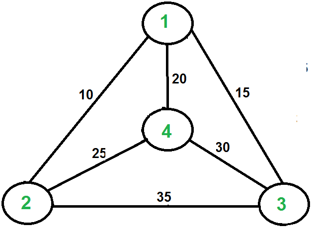
1) Let 1 be the starting and ending point for salesman.
2) Construct MST from with 1 as root using Prim’s Algorithm.
3) List vertices visited in preorder walk of the constructed MST, and add 1 at the end.

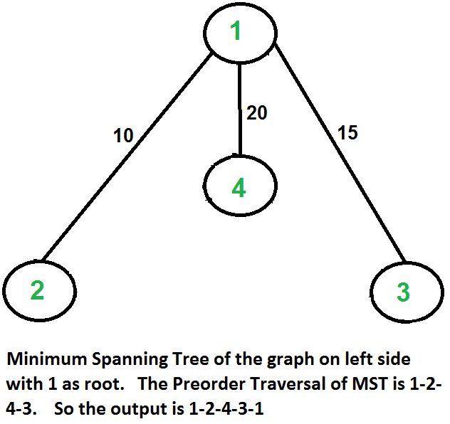
Let us consider the following example. The first diagram is the given graph. The second diagram shows MST constructed with 1 as root. The preorder traversal of MST is 1-2-4-3. Adding 1 at the end gives 1-2-4-3-1 which is the output of this algorithm.

Given a problem like so, we use Prim’s algorithm to create a minimum spanning tree for a weighted undirected graph. It finds a subset of the edges that forms a tree, where the total weight of all the edges in the tree is minimized.

What is Minimum Spanning Tree?

Given a connected and undirected graph, a spanning tree of that graph is a subgraph that is a tree and connects all the vertices together. A single graph can have many different spanning trees. A minimum spanning tree (MST) or minimum weight spanning tree for a weighted, connected and undirected graph is a spanning tree with weight less than or equal to the weight of every other spanning tree. The weight of a spanning tree is the sum of weights given to each edge of the spanning tree.

Prim’s Algorithm

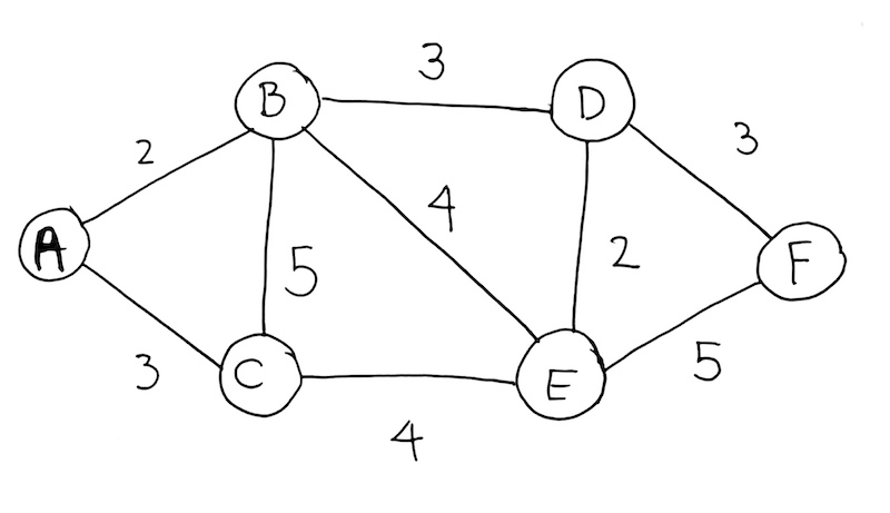
Given Problem

Adjacency List

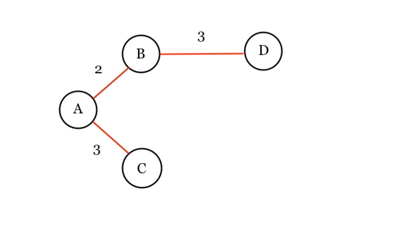
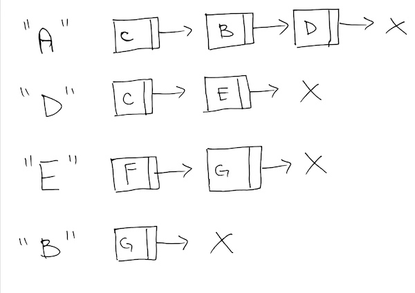
We create an adjacency list. From the diagram, we see that A connects to B and C. So we create key A, and then have it reference a Linked List with nodes B and C.

We see B connects to C, E, and D. So in our adjacency list, we add key B, and have it reference a Linked List with nodes C, E, and D. Repeat until all edges and vertices have been added.

A -> [B] -> [C]
B -> [A] -> [C] -> [E] -> [D]
C -> [A] -> [B] -> [E]
D -> [B] -> [E] -> [F]
E -> [D] -> [E]

The key to picking only the minimum path and getting rid of the rest is accomplished by:

minimum priority queue
visited dictionary to keep track of all visited nodes

The Minimum Queue

We use the minimum priority queue to keep all the edges from nodes that we have visited. We group these edges into this queue, then take the minimum of it. That is how this algorithm picks the minimum path to travel.

Start

We start at node A so we draw it.

We need to process this node A in our min priority queue so we should add it to initialize our queue.

Min Queue: [A]
Visited: {}

Now that the queue has an item, we can start off the process it.

We pop A from the queue to process it.

Min Queue: []
Visited: {}

Has it been visited? No, so we put it in Visited dictionary.
We see from the adjacency list that A connects to B (with distance of 2) and C (with distance of 3).
So we push B and C into our queue.

Min Queue: [ B(A, 2), C(A, 3) ]
Visited: { “A” }

This means that all edges from A is only B and C. And from this group of edges, we use the min priority queue to get the absolute minimum path (which is 2) at node B.

Hence pop B from the queue.

Min Queue: [ C(A, 3) ]
Visited: { “A” }

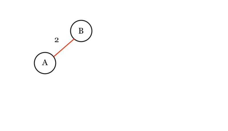
Has B been visited? We look at the Visited dictionary. No. So we then add B to the visited dictionary. . We draw our result:

So we get all its edges from the adjacency list. We see that its nodes D(B, 3), C(B, 5), and E(B, 4).

Min Queue: [ C(A, 3), D(B, 3), C(B, 5), E(B, 4) ]
Visited: { “A”, “B” }

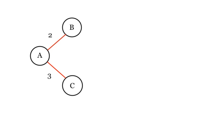
Now we see that the number of available paths have increased to four. We then get the minimum path, which is C(A,3). Has C been visited? Nope, we add it to the Visited dictionary. We draw the path in our diagram.

Then we process it by getting all its edges from the adjacency list. We see that it has node of E(C, 4). We push it onto the Min Queue.
Now, we have 4 available paths from nodes A, B, and C.

Min Queue: [ D(B, 3), C(B, 5), E(B, 4), E(C, 4) ]
Visited: { “A”, “B”, “C” }

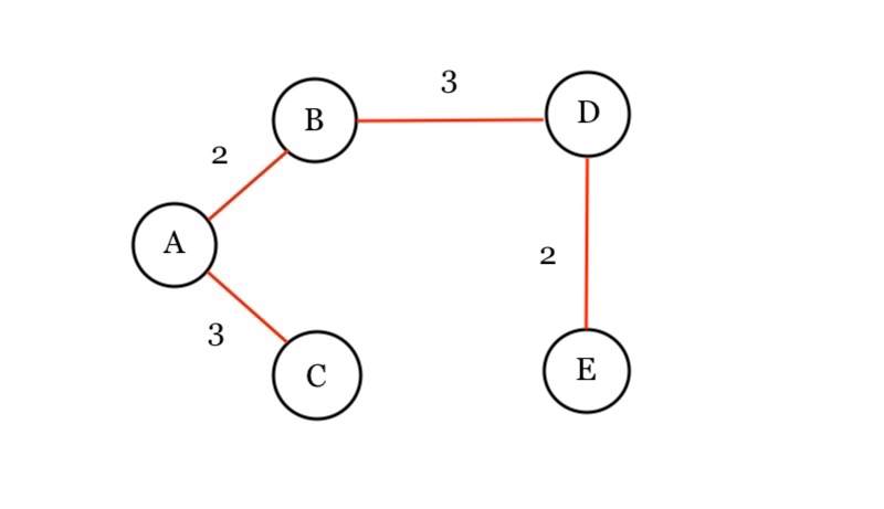
We get minimum of those paths which is D(B,3). Has D been visited? Nope, we add it to the visited dictionary. We draw the path in our diagram.

Then we process D by getting all its edges from the adjacency list. We see that it has node of E(D, 2), F(D, 3). We push it onto the Min Queue.

Min Queue: [ C(B, 5), E(B, 4), E(C, 4), E(D, 2), F(D,3) ]
Visited: { “A”, “B”, “C”, “D” }

We pop the minimum of the priority queue: E(D, 2). Has E been visited? Nope, we add it to the visited dictionary. We draw the path in our diagram.

Then we process E by getting all its edges from the adjacency list. We see that it has node of E(F, 5). We push it onto the Min Queue.

Hence at this point, we have 5 available edges from our visited nodes.

Min Queue: [ C(B, 5), E(B, 4), E(C, 4), F(D,3), E(F, 5) ]
Visited: { “A”, “B”, “C”, “D”, “E” }

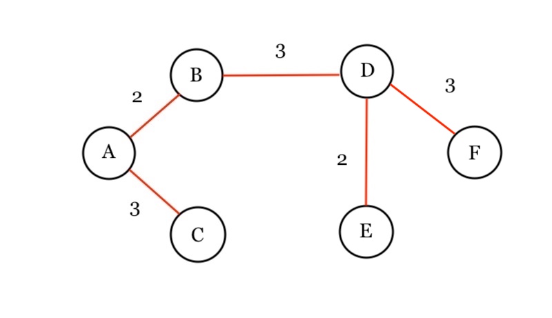
We pop the minimum which is F(D, 3), and process it. Has F been visited? Nope, we add it to the visited dictionary. We update our answer diagram:

From our adjacency list, we see that F does not have a Linked list of edges. Hence, we DO NOT PUSH ANYTHING onto our Priority Queue:

Min Queue: [ C(B, 5), E(B, 4), E(C, 4), E(F, 5) ]
Visited: { “A”, “B”, “C”, “D”, “E”, “F” }

We keep processing. We pop from the minimum queue: E(B, 4) . Has it been visited? Yes, so we skip and continue dequeueing.

Min Queue: [ C(B, 5), E(C, 4), E(F, 5) ]
Visited: { “A”, “B”, “C”, “D”, “E”, “F” }

We pop from the minimum queue: E(C, 4) . Has it been visited? Yes, so we skip and continue dequeueing.

Min Queue: [ C(B, 5), E(F, 5) ]
Visited: { “A”, “B”, “C”, “D”, “E”, “F” }

We pop from the minimum queue: C(B, 5) . Has it been visited? Yes, so we skip and continue dequeueing.

Min Queue: [ E(F, 5) ]
Visited: { “A”, “B”, “C”, “D”, “E”, “F” }

We pop from the minimum queue: E(F, 5) . Has it been visited? Yes, so we skip it and continue.

Now our queue is empty and we’re done.

The answer is:

Dijkstra’s Algorithm

August 18, 2020algorithmsadmin

ref – https://www.tutorialspoint.com/Dijkstra-s-algorithm-in-Javascript

Dijkstra’s Algorithm is used for solving single source shortest path problems. In this algorithm, a single node is fixed as a source node and shortest paths from this node to all other nodes in graph is found.

Minimum priority queue is the most commonly used data structure for implementing Dijkstra’s Algorithm because the required operations to be performed in Dijkstra’s Algorithm match with specialty of a minimum priority queue.

Time complexity of Dijkstra’s algorithm is O(N2) because of the use of doubly nested for loops. It depends on how the table is manipulated.

Dijkstra’s Algorithm cannot be applied on graphs having negative weight function because calculation of cost to reach a destination node from the source node becomes complex.

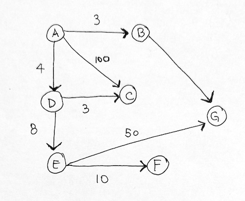
Given nodes: A B C D E F G
and their edges:

“A”, “C”, 100
“A”, “B”, 3
“A”, “D”, 4
“D”, “C”, 3
“D”, “E”, 8
“E”, “F”, 10
“B”, “G”, 9
“E”, “G”, 50

We first draw a node graph diagram of it. Keep in mind that from our adjacency list, if we have arrows pointing to each other from two nodes, it’s undirected. If it’s only from one to the other, then it’s directed. So undirected graphs should have double the # of edges than directed graphs.

In our case, it is a directed graph.

Then we set up the the node/distance/prev chart.
The distance means the shortest distance from the starting node to that node. Right now, we initialize all to infinity.
The prev means the previous node that this node connects to. We maximize as null.

Since our starting node is A, our distance is 0, and prev is A.

node	distance	prev
A	0	A
B	Inf	null
C	Inf	null
D	Inf	null
E	Inf	null
F	Inf	null
G	Inf	null

We then draw the adjacency graph to keep track of all the neighbors of a specific node presented from edges.
For each edge, it creates a neighbor of a node, and we must diagram this in order to keep track.

Finally, we have a queue to get the minimum distance as shall see later.

Start

In our code, we create an instance of our Dijkstra’s Algorithm.

We have the queue ready, so we first push A onto the queue.
queue – [A]

We start by popping the A off the queue and processing it.
queue – []

We look at the unvisited neighbors of A.
Namely, they are C, B, and D.

Distance from A to C is 100. On our chart, distance of A to C is Infinity. 100 < Infinity, so we replace Infinity with 100. Then we push C onto the queue. queue - [C]

node	distance	prev
A	0	A
B	Inf	null
C	100	A
…

Distance from A to B is 3. On the chart, A to B’s distance is Infinity. Is 3 < Infinity? Yes! so we replace the values in the chart, then push node B onto the queue: queue - [B, C]

node	distance	prev
A	0	A
B	3	A
C	100	null
…

Distance from A to D is 4. On the chart A to D’s distance is Infinity. Is 4 < Infinity? Yes! so we replace it on the chart, and push node D onto the queue: queue - [B, D, C]

node	distance	prev
A	0	A
B	3	A
C	100	A
D	4	A

We’ve processed all of node A’s neighbors. (Linked List) Once that’s done. The queue is a priority minimum queue, so we pop the queue to get the minimum distanced node, which is B.

Queue – [D, C]

B with priority of 3

At B, we process all its unvisited neighbors. In the Adjacency list, B is connected to G. B to G is 9. Distance from starting point A to B is 3.
so 3 + 9 = 12. Is 12 < Infinity? yes, so let's update the table.

node	distance	prev
A	0	A
B	3	A
C	100	A
D	4	A
…
G	12	B

Then we push G onto the queue.

Queue – [D, G, C]

Processing D, priority 4

But because D has the minimum distance at 4, we pop it from the queue.

Queue – [G, C]

D has edges to C and E.

Distance from D to C is 3. Distance from start to D 4. Distance from start to C = 3 + 4 = 7. Is 7 < Infinity? Yes, let's update it. Insert C with priority 7 into the queue. Notice we already have priority 100 for C in the queue. We simply replace the value 100 with 7. This is so because we have found a shorter distance than 100.

node	distance	prev
A	0	A
B	3	A
C	7	D
D	4	A
…
G	12	B

We then look at neighbor E. From D to E is 8. From start to D is 4. From start to E is 4 + 8 = 12. Is 12 < Infinity ? Yes, update table. Then push E with priority 12 onto the queue.

node	distance	prev
A	0	A
B	3	A
C	7	D
D	4	A
E	12	D
…
G	12	B

so we’re finished running through all edges for ‘D’.

Queue – [C(7), E(12), G(12)]

Process C with priority of 7

We pop C because it has minimum prioirty.

Queue – [E(12), G(12)]

C has no edges in our Adjacency list, so we skip.

Process G with priority of 12

Queue – [E(12)]

Then we process G with priority of 12. G has no edges in our Adjacency list, so we skip.

Process E with priority of 12

So we then process node E. It has edges F and G.

E to F is 10. Min distance from from start point A to E is 12.
Is 10+12=22 smaller than what’s on our chart? (Infinity) Yes! So we update the chart.

node	distance	prev
A	0	A
B	3	A
C	7	D
D	4	A
E	12	D
F	22	E
G	12	B

Then push F onto the queue.

Queue – [F(22)].

Let’s continue and process G.

E to G is 50. Minimum distance from start to E is 12.
Start to G is 50 + 12 = 62. From our Chart, A to G has 12. Is 62 < 12? No! So we don't update the chart. We do not push G onto the queue. We then pop the queue and continue...

Processing F at priority 22

No edges for F. Queue is empty. WE’re now done.

The final answer is:

node	distance	prev
A	0	A
B	3	A
C	7	D
D	4	A
E	12	D
F	22	E
G	12	B

Where the shortest distance from A to any of the nodes are listed under the distance column.

For example, say I want to know what is the shortest distance from A to G. It is 12 by the way of A, B, G. The 12 shows that A to G takes 12 steps and G’s previous is B. We look at B and its previous is A. So we know that it goes A -> B -> G.

I want to know what is the shortest distance from A to C. Looking at the chart, A to C has min distance of 7, by the way of A, B, C.
C’s previous is B. And B’s previous is A.

Code Explanation

So we have a bunch of dictionaries to represent our chart data. We have everything from distance, prev, and nodes. We have _edges to represent the adjacency list, and _visited to show which ones have been visited.

let _nodes = [];

let distanceArr = {};

let prevArr = {};

let _edges = {};

let _visited = {};

We set up a minimum priority queue.

1	let pq = new PriorityQueue();

And initialize everything first. The start node’s distance is always 0.
We set the other distances to Infinity.
We set the previous nodes to null.
And finally, push the start node onto the queue.

distanceArr[startNode] = 0;

_nodes.forEach(node => {

if (node !== startNode)

distanceArr[node] = Infinity;

prevArr[node] = null;

});

pq.insert(startNode, 0);

So the basic idea here is that we start the algorithm by dequeueing the starting node.
We continue dequeueing from the priority queue until it is empty.

The point of processing each node as they come in is that we get the minimum priority (distance) first.
Then as we process them, we update the chart. We are done when the queue is empty.

let next = pq.remove();

while(next) {

// process the ledges of each node as they come off of the queue

next = pq.remove();

}

As each node with the minimum priority (distance) comes off the queue, we process their edge list. This can be visually seen by the adjacency list. In our case, it is the _edges dictionary.

let currValue = next.value;

// all neighbors of our node

let anEdge = _edges[currValue];

if (!_visited[anEdge.value]) {

let alt = distanceArr[currValue] + anEdge.priority;

if (alt < distanceArr[anEdge.value]) {

// update chart values

// enqueue this node since it has shorter distance

queue.insert(anEdge.value, distanceArr[anEdge.value]);

}

So if an edge has not been visited, we process it.
We the get the minimum distance from starting to current node, and then add the distance of the current edge.
If it’s less than what we have in the chart, we update the chart.

This is to say that we found a shorter way. In this case, we push the current node into the queue along with its distance as the priority.
Due to the queue being a minimum priority queue, it will always process the shortest distance nodes.

If it’s not, then this way is longer, and we don’t care for it.

Source Code

Node, Linked List and Minimum Priority Queue

100

101

102

103

104

105

106

107

108

109

110

111

112

113

114

115

116

117

118

119

120

121

122

123

124

125

126

127

128

129

130

131

132

133

134

135

136

137

138

139

140

141

142

143

144

145

146

147

148

149

150

151

152

153

154

155

156

157

158

159

160

161

162

163

class Node {

constructor(val, priority) {

this.value = val;

this.priority = priority;

this.next = null;

}

print() {

console.log(`${this.value} (${this.priority})`);

}

let createLinkedListInstance = (function LinkedList() {

let head = null;

let tail = null;

let iterator = null;

return new class LinkedList {

add = function(value, priority) {

if (!head && !tail) {

head = new Node(value, priority, null);

tail = head;

iterator = head;

} else {

tail.next = new Node(value, priority, null);

tail = tail.next;

}

print = () => {

console.log(`--- printing Linked List ---`);

for (let tmp = head; tmp != null; tmp = tmp.next) {

console.log(tmp);

}

next = () => {

if (iterator) {

let tmp = iterator;

iterator = iterator.next;

return tmp;

} else {

return null;

}

hasNext = () => { return iterator ? true : false; }

resetIterator = () => { iterator = head; }

}

});

class PriorityQueue {

constructor() {

this.heap = []; // array, with first null element

}

print(index) {

console.log("----- PRINTING HEAP --------")

//let next = 2 * index + 1;

//console.log("***")

for (let v = 0; v < this.heap.length; v++) {

//if (v === next) {

//console.log("\n***");

// then recalculate

//next = 2 * v + 1;

//}

//process.stdout.write(`${this.heap[v].value}, ${this.heap[v].priority} | `);

console.log(`${this.heap[v].value}, ${this.heap[v].priority} | `);

}

console.log("\n--------- finished printing heap -----------");

}

// worse case, number of levels, translates to O(log n)

insert (value, priority) {

const newNode = new Node(value, priority);

this.heap.push(newNode);

let currentNodeIdx = this.heap.length-1;

let currentNodeParentIdx = Math.ceil( (currentNodeIdx-2) / 2);

while(this.heap[currentNodeParentIdx] &&

newNode.priority < this.heap[currentNodeParentIdx].priority) {

const parent = this.heap[currentNodeParentIdx];

this.heap[currentNodeParentIdx] = newNode;

this.heap[currentNodeIdx] = parent;

currentNodeIdx = currentNodeParentIdx;

currentNodeParentIdx = Math.ceil((currentNodeIdx-2)/2);

}

} // insert

getLeftChildIndex(currentIndex) {return 2 * currentIndex + 1;}

getRightChildIndex(currentIndex) {return 2 * currentIndex + 2;}

getLeftChild(currentIndex) {return this.heap[this.getLeftChildIndex(currentIndex)];}

setLeftChild(currentIndex, newNode) {this.heap[this.getLeftChildIndex(currentIndex)] = newNode;}

getRightChild(currentIndex) {return this.heap[this.getRightChildIndex(currentIndex)];}

setRightChild(currentIndex, newNode) { this.heap[this.getRightChildIndex(currentIndex)] = newNode;}

getCurrentNode(currentIndex) { return this.heap[currentIndex]; }

setCurrentNode(currentIndex, newNode) {this.heap[currentIndex] = newNode;}

exchangeCurrentAndLeftChild(currentIndex, left) {

let temp = this.getCurrentNode(currentIndex);

this.setCurrentNode(currentIndex, left);

this.setLeftChild(currentIndex, temp);

}

exchangeCurrentAndRightChild(currentIndex, right) {

let temp = this.getCurrentNode(currentIndex);

this.setCurrentNode(currentIndex, right);

this.setRightChild(currentIndex, temp);

}

topToBottomHeapify(currentIndex) {

let current = this.getCurrentNode(currentIndex);

if (!current) {return null;} else {

console.log(`processing index ${currentIndex} for value: ${this.heap[currentIndex].value}`);

}

let left = this.getLeftChild(currentIndex);

let right = this.getRightChild(currentIndex);

if (left && !right && left.priority < current.priority) {

this.exchangeCurrentAndLeftChild(currentIndex, left);

} else if (!left && right && right.priority < current.priority) {

this.exchangeCurrentAndRightChild(currentIndex, right);

} else if (left && right && (left.priority < current.priority || right.priority < current.priority)) {

console.log(`both left and right exists: ${left.priority}, ${right.priority}, and one of them is larger than parent`);

if (left.priority < right.priority) {

this.exchangeCurrentAndLeftChild(currentIndex, left);

} else {

this.exchangeCurrentAndRightChild(currentIndex, right);

}

this.topToBottomHeapify(2*currentIndex+1);

this.topToBottomHeapify(2*currentIndex+2);

}

remove() {

let toProcess = this.heap[0];

if (toProcess) {

console.log(`√ Processing task ${toProcess.value}`);

this.heap[0] = this.heap[this.heap.length-1];

this.heap.pop();

this.topToBottomHeapify(0);

return toProcess;

} else {

console.log('now empty');

return null;

}

export { Node };

export { PriorityQueue };

export { createLinkedListInstance };

Dijkstra’s Algorithm

100

101

102

103

104

105

106

107

108

109

110

111

112

113

114

115

116

117

118

119

120

121

122

123

124

125

126

127

128

129

130

131

132

133

134

135

136

137

138

139

140

141

let l = console.log;

let DijkstraAlgo = (function() {

let _edges = {};

let _nodes = [];

let _visited = {};

return new class dijkstra {

constructor() {}

addNode = value => { _nodes.push(value); }

addDirectedEdge = (fromValue, toValue, priority) => {

let list = _edges[fromValue];

if (!list) {

_edges[fromValue] = createLinkedListInstance();

_edges[fromValue].add(toValue, priority);

} else { // neighbors exist

_edges[fromValue].add(toValue, priority);

}

dijkstraAlgorithm(startNode) {

let distanceArr = {};

let prevArr = {};

let pq = new PriorityQueue();

distanceArr[startNode] = 0;

pq.insert(startNode, 0);

_nodes.forEach(node => {

if (node !== startNode)

distanceArr[node] = Infinity;

prevArr[node] = null;

});

l(_nodes);

l(distanceArr);

l(prevArr);

let next = pq.remove();

while(next) {

let currValue = next.value;

console.log(`------------------- processing LIST of ${currValue} via priority ${next.priority}------------------`);

// all neighbors of our node

let edges = _edges[currValue];

if (edges) {

edges.print();

while (edges.hasNext()) {

let anEdge = edges.next();

if (!_visited[anEdge.value]) {

console.log(`neighbor name ${anEdge.value}, priority of neighbor ${anEdge.priority}, dist from ${currValue} to start point ${distanceArr[currValue]}`);

let alt = distanceArr[currValue] + anEdge.priority;

console.log(`distance from starting ${startNode} to ${anEdge.value} is ${alt}`);

console.log(`Is ${alt} < ${distanceArr[anEdge.value]} ?`)

// value is smaller than what's on the board

if (alt < distanceArr[anEdge.value]) {

// update our board so it has shorter value

distanceArr[anEdge.value] = alt;

// update the prev so we know which is the previous node

prevArr[anEdge.value] = currValue;

// insert all edges into our priority queue

// we put distance as priority so that smallest priority

// gets processed first

console.log(`Yes, insert ${anEdge.value} with priority ${distanceArr[anEdge.value]} into queue`)

pq.insert(anEdge.value, distanceArr[anEdge.value]);

}

_visited[currValue] = true;

l(distanceArr);

l(prevArr);

} else {

console.log(`No edges nodes for node ${currValue}`);

}

next = pq.remove();

console.log('==================================================');

}

l(distanceArr);

}

print = () => {

l(_nodes);

for (var key in _edges) {

if (Object.prototype.hasOwnProperty.call(_edges, key)) {

// do stuff

console.log('printing for key: ' + key);

_edges[key].print();

}

});

let g = new DijkstraAlgo();

g.addNode("A");

g.addNode("B");

g.addNode("C");

g.addNode("D");

g.addNode("E");

g.addNode("F");

g.addNode("G");

g.addDirectedEdge("A", "C", 100);

g.addDirectedEdge("A", "B", 3);

g.addDirectedEdge("A", "D", 4);

g.addDirectedEdge("D", "C", 3);

g.addDirectedEdge("D", "E", 8);

g.addDirectedEdge("E", "F", 10);

g.addDirectedEdge("B", "G", 9);

g.addDirectedEdge("E", "G", 50);

g.dijkstraAlgorithm("A");

Graphs Problems (networks, routes/paths, scheduling…etc)

August 12, 2020algorithms, Computer Scienceadmin

ref –

https://www.geeksforgeeks.org/depth-first-search-or-dfs-for-a-graph/
https://www.geeksforgeeks.org/breadth-first-search-or-bfs-for-a-graph/
https://stackoverflow.com/questions/14720691/whats-the-purpose-of-bfs-and-dfs

BFS and DFS are graph search algorithms that can be used for a variety of different purposes. Many problems in computer science can be thought of in terms of graphs. For example, analyzing networks, mapping routes, and scheduling are graph problems. Graph search algorithms like breadth-first search are useful for analyzing and solving graph problems.

One common application of the two search techniques is to identify all nodes that are reachable from a given starting node. For example, suppose that you have a collection of computers that each are networked to a handful of other computers. By running a BFS or DFS from a given node, you will discover all other computers in the network that the original computer is capable of directly or indirectly talking to. These are the computers that come back marked.

BFS specifically can be used to find the shortest path between two nodes in an unweighted graph. Suppose, for example, that you want to send a packet from one computer in a network to another, and that the computers aren’t directly connected to one another. Along what route should you send the packet to get it to arrive at the destination as quickly as possible? If you run a BFS and at each iteration have each node store a pointer to its “parent” node, you will end up finding route from the start node to each other node in the graph that minimizes the number of links that have to be traversed to reach the destination computer.

DFS is often used as a subroutine in more complex algorithms. For example, Tarjan’s algorithm for computing strongly-connected components is based on depth-first search. Many optimizing compiler techniques run a DFS over an appropriately-constructed graph in order to determine in which order to apply a specific series of operations. Depth-first search can also be used in maze generation: by taking a grid of nodes and linking each node to its neighbors, you can construct a graph representing a grid. Running a random depth-first search over this graph then produces a maze that has exactly one solution.

This is by no means an exhaustive list. These algorithms have all sorts of applications, and as you start to explore more advanced algorithms you will often find yourself relying on DFS and BFS as building blocks. It’s similar to sorting – sorting by itself isn’t all that interesting, but being able to sort a list of values is enormously useful as a subroutine in more complex algorithms.

We use graphs to present connected nodes.

Graph consist of nodes and edges.

Adjacent – if two nodes are directed connected. They are neighbors.

If it’s a directed graph, and John has an arrow towards Bob, then John is adjacent to Bob. But opposite not true.

Edges also have a weight. If two people interact a lot, they can have a higher weighted edge.

Finding two shortest path to two nodes.

Adjacency Matrix

An adjacency list is a collection of unordered lists used to represent a finite graph.

Each list describes the set of neighbors of a vertex in the graph.

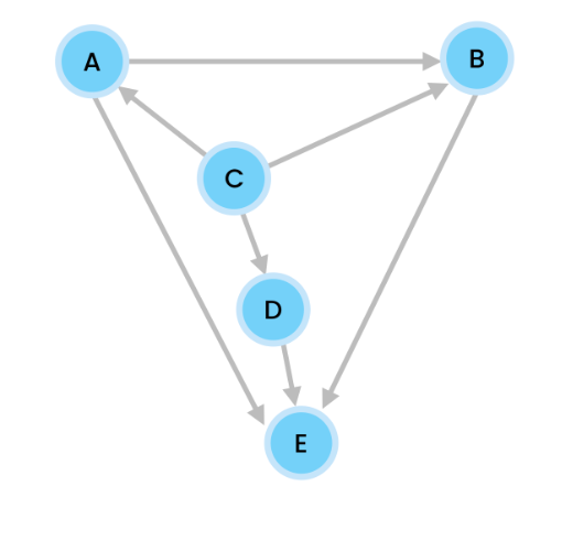
Let’s do Depth First Search on our example graph

The idea is to go forward in depth while there is any such possibility. If not then backtrack.

Whenever we push an unvisited node, we print it.

Before we start, there are two assumptions:

– we start at node C
– nodes are inserted in alphabetical order.

We use a stack.

So we start at C. We push C onto our stack, and print it.

stack: C
output: C

C is connected to three nodes, A, B, and D. We do this alphabetically so we push A onto the stack, and print it.

stack: C A
output: C A

At A, we have two nodes, B and E. We push B onto our stack, and print it.

stack: C A B
output: C A B

B has one neighbor E. So we push E onto the stack, and print it.

stack: C A B E
output: C A B E

Since E has no connecting neighbors, we pop it.

stack: C A B
output: C A B E

We are now at B. B’s only neighbor of E has already been visited so we pop B.

stack: C A
output: C A B E

A’s neighbors B and E have all been visited. So we push A.

stack: C
output: C A B E

Now we’re at C.

C’s A has been visited, and B has also been visited. But B is unvisited so we push D onto the stack, then print it.

stack: C D
output: C A B E D

D has no unvisited nodes so we pop it.

stack: C
output: C A B E D

C has no unvisited nodes so we pop.

stack:
output: C A B E D

Stack is empty so we’re done.

Source Code

We create a list that has a tail pointing to the latest item we insert. That way, everything is order. Whatever you added first, will be processed first as head is referencing it. Tail will always reference the very last item you add.

let l = console.log;

function Node(data, next) {

this.data = data;

this.next = next;

this.print = function(){

console.log(`Node - ${this.data}`);

}

let createLinkedListInstance = (function LinkedList() {

let head = null;

let tail = null;

let iterator = null;

return new class LinkedList {

add = function(value) {

if (!head && !tail) {

head = new Node(value, null);

tail = head;

iterator = head;

} else {

tail.next = new Node(value, null);

tail = tail.next;

}

print = () => {

for (let tmp = head; tmp != null; tmp = tmp.next) {

tmp.print();

}

next = () => {

if (iterator) {

let tmp = iterator;

iterator = iterator.next;

return tmp;

} else {

return null;

}

hasNext = () => {

return iterator ? true : false;

}

resetIterator = () => {

iterator = head;

}

});

Create a Graph with x number of nodes.

let createGraphInstance = (function(numOfVertices) {

// private properties

let output = [];

console.log(`create a graph with ${numOfVertices} nodes`);

var numOfNodes = numOfVertices;

var adj = [];

We use recursion on the local stack frame in order to simulate a stack.

Each list that is referenced by an Adj[key] is pushed onto the stack. As we process each node down this list, we get more keys, say key2.

We then push list referenced by Adj[key2] onto the local stack frame by recursively calling the function. We keep doing this until we exhaust this list.

Then the function gets popped off the local stack frame.

let _dfsUtil = function(fromNodeKey, visitedArr) {

l(`PUSH adj[${fromNodeKey}] onto stack`);

output.push(fromNodeKey);

visitedArr[fromNodeKey] = true;

let list = adj[fromNodeKey];

while (list && list.hasNext()) {

let node = list.next();

let nodeKey = node.data;

if (!visitedArr[nodeKey]) {

_dfsUtil(nodeKey, visitedArr);

} else {

l(`node ${fromNodeKey} - `, `already processed ${nodeKey}`);

}

l(`POP adj[${fromNodeKey}] from stack`);

} //

We look at our graph, and add the neighbors that are connected to our node. We always do this before we run the DFS function.

return new class Graph {

// public, prototype

addEdge = function(fromNodeKey, toNodeKey) {

let list = adj[fromNodeKey];

if (!list) {

l('creating new');

adj[fromNodeKey] = createLinkedListInstance();

if (toNodeKey) {

adj[fromNodeKey].add(toNodeKey);

}

} else {

list.add(toNodeKey);

}

} //

After adding all the nodes, and specifying how many nodes we have in the constructor, we are ready to call this function.

// recursion is the stack

dfs(nodeNumber) {

l(`starting from node ${nodeNumber}`);

let visited = new Array(numOfNodes);

_dfsUtil(nodeNumber, visited);

}

print our adjacency list and the lists that they contain

print = () => {

l(`-- printing --`);

let allKeys = Object.keys(adj);

l(allKeys);

for (const key of allKeys) {

l(`------ ${key} --------`);

adj[key].print();

}

print the output array

printOutput = () => {

l(output);

}

});

let g = createGraphInstance(5);

g.addEdge('a', 'b');

g.addEdge('a', 'e');

g.addEdge('b', 'e');

g.addEdge('c', 'a');

g.addEdge('c', 'b');

g.addEdge('c', 'd');

g.addEdge('d', 'e');

g.addEdge('e');

g.print();

// let's do this starting from node 2

g.dfs('c');

g.printOutput();

Breadth First Search on the graph

The trick is that you visit a dequeued node. If that node is NOT visited, we add its neighbors to the queue. If that node HAS ALREADY BEEN visited, we keep dequeueing.

We start at C, so we add C to the queue.

queue: [C]

We remove C from the queue and visit it.

output: C
queue: []

We now must add C’s unvisited neighbors tot he queue (in alphabetical order).

output: C
queue: [A, B, D]

We visit A, and remove it from the queue.

output: C A
queue: [B, D]

Since we visited A, we must add A’s unvisited neighbors to the queue. Those neighbors are B and E.

output: C A
queue: [B, D, B, E]

We visit B, and dequeue it.

output: C A B
queue: [D, B, E]

Since we visited B, let’s look at its neighbors. It has one neighbor E. Let’s add it to the queue.

output: C A B
queue: [D, B, E, E]

No we visit D and print. Then dequeue it.

output: C A B D
queue: [B, E, E].

since we visited D, we must add its unvisited neighbors E.

output: C A B D
queue: [B, E, E, E]

Now we dequeue B, but we see that we have already visited it.

output: C A B D
queue: [E, E, E]

We then dequeue E. It has not been visited so we output it.

output: C A B D E
queue: [E, E]

E has no neighbors so we don’t add anything to the queue.

We then dequeue again. Has no neighbors so we continue to dequeue.

output: C A B D E
queue: [E]

Finally, we dequeue the last E. It has already been printed. And it has no neighbors. The queue is now empty so we’re done.

output: C A B D E
queue: []

We first create a queue.

let createQueue = (function Queue() {

let head = null;

let tail = null;

return new class Queue {

enqueue = value => {

if (!head && !tail) {

head = new Node(value, null);

tail = head;

} else {

tail.next = new Node(value, null);

tail = tail.next;

}

dequeue = () => {

let tmp = head;

head = head.next;

if (!head) { tail = null; }

return tmp;

}

size = () => {

let tmp = head;

let count = 0;

while (tmp) {

count++;

tmp = tmp.next;

}

return count;

}

});

We use the Linked List from the previous example.

So with Breadth first traversal of the graph, the trick is that we start at the initial node.

We then take all the neighbors of that node and add them to the queue. Once we added all those neighbors, we pop the initial node, and then move on to process the next one in queue.

let createBreadthFirstSearchForGraph = (function(numOfVertices) {

// private here

let output = [];

var numOfNodes = numOfVertices;

var adj = [];

return new class BFSGraph {

addEdge = function(fromNodeKey, toNodeKey) {

let list = adj[fromNodeKey];

if (!list) {

l('creating new');

adj[fromNodeKey] = createLinkedListInstance();

if (toNodeKey) {

adj[fromNodeKey].add(toNodeKey);

}

} else {

list.add(toNodeKey);

}

} //

So as you can see, we give it an initial key to start from. In our case it is ‘c’. So fromNodeKey is ‘c’.
We then keep track if they are visited or not via a visited array.

Initially, we only have one node in the queue. So we start processing the while loop. We pop the ‘c’ node and then push all the nodes from its neighbors via an inner while loop.

In this inner loop, we check to see if the key has been processed by associative array access on the visited array. If it has not been visited, we mark it visited and then add it onto our queue to be processed later.

bfs = fromNodeKey => {

let visited = new Array(numOfNodes);

let queue = createQueue();

visited[fromNodeKey] = true;

l(visited);

queue.enqueue(fromNodeKey);

l(queue);

let s;

while (queue.size() != 0) {

// 2) we then process them one by one

// base case is whatever node you want to start from

s = queue.dequeue();

output.push(s.data);

let list = adj[s.data];

// 1) we push all neighbors of current node onto the queue

while (list.hasNext()) {

let node = list.next();

let nodeKey = node.data;

if (!visited[nodeKey]) {

visited[nodeKey] = true;

queue.enqueue(nodeKey);

}

....

}

});

Source Code

Depth First Graph Traversal

100

101

102

103

104

105

106

107

108

109

110

111

112

113

114

115

116

117

118

119

120

121

122

123

124

125

126

127

128

129

130

131

132

133

134

135

136

137

138

139

140

141

142

143

144

145

146

147

148

149

150

151

152

153

let l = console.log;

function Node(data, next) {

this.data = data;

this.next = next;

this.print = function(){

console.log(`Node - ${this.data}`);

}

let createLinkedListInstance = (function LinkedList() {

let head = null;

let tail = null;

let iterator = null;

return new class LinkedList {

add = function(value) {

if (!head && !tail) {

head = new Node(value, null);

tail = head;

iterator = head;

} else {

tail.next = new Node(value, null);

tail = tail.next;

}

print = () => {

for (let tmp = head; tmp != null; tmp = tmp.next) {

tmp.print();

}

next = () => {

if (iterator) {

let tmp = iterator;

iterator = iterator.next;

return tmp;

} else {

return null;

}

hasNext = () => {

return iterator ? true : false;

}

resetIterator = () => {

iterator = head;

}

});

let createGraphInstance = (function(numOfVertices) {

// private properties

let output = [];

console.log(`create a graph with ${numOfVertices} nodes`);

var numOfNodes = numOfVertices;

var adj = [];

let _dfsUtil = function(fromNodeKey, visitedArr) {

l(`PUSH adj[${fromNodeKey}] onto stack`);

output.push(fromNodeKey);

visitedArr[fromNodeKey] = true;

let list = adj[fromNodeKey];

while (list && list.hasNext()) {

let node = list.next();

let nodeKey = node.data;

if (!visitedArr[nodeKey]) {

_dfsUtil(nodeKey, visitedArr);

} else {

l(`node ${fromNodeKey} - `, `already processed ${nodeKey}`);

}

l(`POP adj[${fromNodeKey}] from stack`);

} //

return new class Graph {

// public, prototype

addEdge = function(fromNodeKey, toNodeKey) {

let list = adj[fromNodeKey];

if (!list) {

l('creating new');

adj[fromNodeKey] = createLinkedListInstance();

if (toNodeKey) {

adj[fromNodeKey].add(toNodeKey);

}

} else {

list.add(toNodeKey);

}

} //

// recursion is the stack

dfs(nodeNumber) {

l(`starting from node ${nodeNumber}`);

let visited = new Array(numOfNodes);

_dfsUtil(nodeNumber, visited);

}

print = () => {

l(`-- printing --`);

let allKeys = Object.keys(adj);

l(allKeys);

for (const key of allKeys) {

l(`------ ${key} --------`);

adj[key].print();

}

printOutput = () => {

l(output);

}

});

let g = createGraphInstance(5);

g.addEdge('a', 'b');

g.addEdge('a', 'e');

g.addEdge('b', 'e');

g.addEdge('c', 'a');

g.addEdge('c', 'b');

g.addEdge('c', 'd');

g.addEdge('d', 'e');

g.addEdge('e');

g.print();

// let's do this starting from node 2

g.dfs('c');

g.printOutput();

Breadth First Traversal for Graphs

Linked List used is same as above.

100

101

102

103

104

105

106

107

108

109

110

111

112

113

114

115

116

117

118

119

120

121

122

123

124

125

126

127

128

let createQueue = (function Queue() {

let head = null;

let tail = null;

return new class Queue {

enqueue = value => {

if (!head && !tail) {

head = new Node(value, null);

tail = head;

} else {

tail.next = new Node(value, null);

tail = tail.next;

}

dequeue = () => {

let tmp = head;

head = head.next;

if (!head) { tail = null; }

return tmp;

}

size = () => {

let tmp = head;

let count = 0;

while (tmp) {

count++;

tmp = tmp.next;

}

return count;

}

});

let createBreadthFirstSearchForGraph = (function(numOfVertices) {

// private here

let output = [];

var numOfNodes = numOfVertices;

var adj = [];

return new class BFSGraph {

addEdge = function(fromNodeKey, toNodeKey) {

let list = adj[fromNodeKey];

if (!list) {

l('creating new');

adj[fromNodeKey] = createLinkedListInstance();

if (toNodeKey) {

adj[fromNodeKey].add(toNodeKey);

}

} else {

list.add(toNodeKey);

}

} //

bfs = fromNodeKey => {

let visited = new Array(numOfNodes);

let queue = createQueue();

visited[fromNodeKey] = true;

l(visited);

queue.enqueue(fromNodeKey);

l(queue);

let s;

while (queue.size() != 0) {

// 2) we then process them one by one

// base case is whatever node you want to start from

s = queue.dequeue();

output.push(s.data);

let list = adj[s.data];

// 1) we push all neighbors of current node onto the queue

while (list.hasNext()) {

let node = list.next();

let nodeKey = node.data;

if (!visited[nodeKey]) {

visited[nodeKey] = true;

queue.enqueue(nodeKey);

}

print = () => {

l(`-- printing --`);

let allKeys = Object.keys(adj);

l(allKeys);

for (const key of allKeys) {

l(`------ ${key} --------`);

adj[key].print();

}

printOutput = () => {

l(output);

}

});

let b = createBreadthFirstSearchForGraph(5);

b.addEdge('a', 'b');

b.addEdge('a', 'e');

b.addEdge('b', 'e');

b.addEdge('c', 'a');

b.addEdge('c', 'b');

b.addEdge('c', 'd');

b.addEdge('d', 'e');

b.addEdge('e');

b.print();

b.bfs('c');

b.printOutput();

Mosh Trees Tutorial

August 6, 2020algorithms, Computer Scienceadmin

Non Linear Data structures – trees

Tree is a data structure that stores element in a hierarchy.

Root – Top node of tree
Root is parent of its children.
Each node can have up to two nodes…this is called a binary tree.

Trees

– represent hierarchical data
– databases
– autocompletion
– compilers (syntax tree to parse expressions)
– compression (JPEG, MP3)

left < node < right At every step of comparison, we throw away half of the tree. This is what we call Logarithmic Time

Lookup
O(log n)

Inserting node
Finding a Node O(log n) + Inserting Node O(1) = O(log n)

Delete Node
O(log n)

Depth First Search (DFS)

pre-order – (left of node)
in-order – (bottom of node) ascending order
post-order – (right of node)

Breadth First – Level by level (BFS)

Recursion

Iteration – loops.
Recursion – no loops.

Base condition terminates Recursion.

Depths and Height

Depths starts at the root

Depths of root is 0. As it goes deeper, it increases.
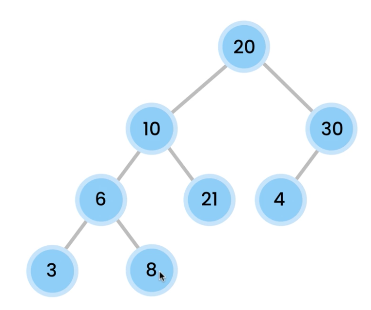
Depth of 10 is 1.
Depth of 21 is 2.
Depth of 8 is 3.

Depth – # of edges from root to target node.

Height is opposite of depth.

Height starts at the leaf

Height of leafs are 0.
As we go up, height increases. Longest path from target node to leaf.

Height of 6 is 1.

Height of 30 is 1.

Height of 10 is 2. We actually have 3 different paths. 3 to 10. 8 to 10. 21 to 10. Longest path is 2.

Height of 20 is 3, because it’s the longest path.

1 + max(height(L) + height(R))

Post Traversal – visit all leaves first

function getHeight() {

if (!root) return 0;

return height(root);

}

// private

height(node) {

if (!node.left && !node.right) {

return 0;

}

return 1 + Math.max(

height(node.left),

height(node.right));

}

Find minimum value in BST

If it’s a standard BST, use recursion, and get leftmost leaf.

function min(node) { // O(log n)

if (!node.left) {

return node.value;

} else {

return min(node.left);

}

But if its NOT a BST, values are all over the place, so

function min (node) { // O(n)

if (!node) return 0;

if (!node.left && !node.right) return node.value;

let childrenMin = Math.min(node.left, node.right);

return Math.min(childrenMin, node.value);

}

Exercises

– height of tree. return Math.max of left subtree and right subtree. That way, you get the height at the root.

– # of nodes at distance k. simple pre-order and print.

– isBST? pass in parameter min, max. Make sure node value stays within range. If not, false. Kick off with -Infinity and +Infinity.

Minimum – isBST? if yes, get leftmost. If not, then must have parameter reference and recurse down, do compare with every value.

Maximum – isBST? if yes, get rightmost. If not, then must have parameter reference and recurse down, do compare with every value.

– Are the two tree equal (Equality Check)?

– traverse BST (Level Order Traversal)

for i to height of tree
let arr = getNodesAtDistance(i)
for j to arr.length
log arr[j];

Additional exercises

1- Implement a method to calculate the size of a binary tree. Solution: Tree.size()

2- Implement a method to count the number of leaves in a binary tree. Solution: Tree.countLeaves()

4- Implement a method to check for the existence of a value in a binary tree using recursion. Compare this method with the find() method. The find() method does the same job using iteration. Solution: Tree.contains()

5- Implement a method to check to see if two values are siblings in a binary tree. Solution: Tree.areSibling()

6- Implement a method to return the ancestors of a value in a List. Solution: Tree.getAncestors()

SOLUTION

100

101

102

103

104

105

106

107

108

109

110

111

112

113

114

115

116

117

118

119

120

121

122

123

124

125

126

127

128

129

130

131

132

133

134

135

136

137

138

139

140

141

142

143

144

145

146

147

148

149

150

151

152

153

154

155

156

157

158

159

160

161

162

163

164

165

166

167

168

169

170

171

172

173

174

175

176

177

178

179

180

181

182

183

184

185

186

187

188

189

190

191

192

193

194

195

196

197

198

199

200

201

202

203

204

205

206

207

208

209

210

211

212

213

214

215

216

217

218

219

220

221

222

223

224

225

226

227

228

229

230

231

232

233

234

235

236

237

238

239

240

class Node {

constructor(newData, newLeft, newRight) {

this.left = newLeft;

this.right = newRight;

this.data = newData;

}

print = () => {

console.log(this.data);

}

class Tree {

constructor() {

var root = null;

this.getRoot = function() {return root;}

this.addData = function (data) {

if (root == null) {

root = new Node(data, null, null);

} else {

_addNode(root, new Node(data, null, null));

}

function _addNode(node, toAddNode) {

if (node == null) { return toAddNode;}

if (toAddNode.data > node.data) {

node.right = _addNode(node.right, toAddNode);

} else {

node.left = _addNode(node.left, toAddNode);

}

return node;

}

this.printInOrder = function() {

console.log(`-- printing nodes in order --`);

if (root==null) {

console.log('nothing in tree');

} else {

_inOrderTraversal(root, function(node){

node.print();

});

}

console.log(`-----------------------------`);

}

function _inOrderTraversal(node, callback) {

if (node == null) return;

_inOrderTraversal(node.left, callback);

callback(node);

_inOrderTraversal(node.right, callback);

}

this.getHeightOfTree = function() {

// return Math.max of left subtree and right subtree.

// That way, you get the height at the root.

if (!root) return 0;

return height(root);

}

function height(node) {

// base case

if (!node.left && !node.right) return 0;

let heightOfLeft = (node.left) ? 1+height(node.left) : 0;

let heightOfRight = (node.right) ? 1+height(node.right) : 0;

return Math.max(heightOfLeft, heightOfRight);

}

// isBST? pass in parameter min, max. Make sure node value stays within range.

// If not, false. Kick off with -Infinity and +Infinity.

this.isBST = function() {

return nodeWithMinMax(-Infinity, root, Infinity);

}

function nodeWithMinMax(smallerValue, node, largerValue) {

if (!node) { return true; } // base case

let bLeft = nodeWithMinMax(smallerValue, node.left, node.data);

let bRight = nodeWithMinMax(node.data, node.right, largerValue);

return bLeft && bRight && (node.data > smallerValue && node.data < largerValue);

}

// used to make a Binary Tree that is not ordered (non-BST)

this.errorTree = function () {

let Three = new Node(1, null, null)

let Eleven = new Node(11, null, Three)

let Two = new Node(2, null, null);

root = new Node(99, new Node(12, Two, null), Eleven);

}

// Nodes at K distance. Given distance from the root.

// print all nodes with distance 3 from root. You print the nodes. Not the whole subtree.

this.nodesWithKDistanceFromRoot = function(k) {

let queue = [];

distanceK(root, 0, k, queue);

return queue;

}

function distanceK(node, count, k, queue) {

if (node == null) {return;}

if (count == k) {

//node.print();

queue.push(node);

return;

}

distanceK(node.left, count+1, k, queue);

distanceK(node.right, count+1, k, queue);

}

// Minimum – isBST? if yes, get leftmost. If not, then must have parameter reference and recurse down, do compare with every value.

this.getMinimumValue = function() {

if (this.isBST()) {

return getLeftMostNode(root).data;

} else {

return getMinInNonBST(root, Infinity);

}

function getLeftMostNode(node) {

return (node.left) ? getLeftMostNode(node.left) : node;

}

function getMinInNonBST(node, min) {

if (!node) return Infinity;

min = Math.min(node.data, min);

if (!node.left && !node.right) return min;

return Math.min(getMinInNonBST(node.left, min), getMinInNonBST(node.right, min));

}

this.getMaximumValue = function() {

if (this.isBST()) {

return getRightMostNode(root).data;

} else {

return getMaxInNonBST(root, -Infinity);

}

function getRightMostNode(node) {

return (node.right) ? getRightMostNode(node.right) : node;

}

function getMaxInNonBST(node, max) {

if (!node) return -Infinity;

max = Math.max(node.data, max);

if (!node.left && !node.right) return max;

return Math.max(getMaxInNonBST(node.left, max), getMaxInNonBST(node.right, max));

}

this.getBSTatLvl = function(level) {

for (let i = 0; i <= level; i++) {

let q = this.nodesWithKDistanceFromRoot(i);

console.log(`-- Depth of ${i} --`);

q.forEach(item => console.log(item.data));

}

this.getLeaves = function() { // done

let ht = this.getHeightOfTree(root);

return this.nodesWithKDistanceFromRoot(ht);

}

this.treeSize = function() { // done

let ht = this.getHeightOfTree(root);

let total = [];

for (let i = 0; i <= ht; i++) {

let q = this.nodesWithKDistanceFromRoot(i);

total = total.concat(q);

}

return total.length;

}

this.findValue = function(value, callback) { // done

return checkValue(root, value, callback);

}

function checkValue(node, value, callback) {

if (!node) return null;

else if (node.data == value) {

callback(node);

return node;

}

let left = checkValue(node.left, value, callback);

let right = checkValue(node.right, value, callback);

return (left || right);

}

this.areSiblings = function(first, second) { // done

return checkSib(root, first, second)

}

function checkSib(node, first, second) {

if (!node.left || !node.right) { return false }

let bChildren = checkSib(node.left, first, second) || checkSib(node.right, first, second);

if (node.left && node.right) {

return (node.left.data == first && node.right.data == second) || bChildren;

}

return bChildren;

}

function f(node, value, ancestorList) {

if (!node) {return false;}

if (node && (node.data === value)) { // when found, we immediately return true

return true;

} else { // if not found, we recruse down

let left = f(node.left, value, ancestorList);

// we check if it is an ancestor. If so, we add to the list

if (left) {

ancestorList.push(node);

return true;

}

let right = f(node.right, value, ancestorList);

// we check if it is an ancestor. If so, we add to the list

if (right) {

ancestorList.push(node);

return true;

}

// if not ancestor, return false, which means don't add to list.

return false;

}

this.getAncestors = function(value) {

let ancestors = [];

f(root, value, ancestors);

return ancestors;

}

} // constructor

// prototype functions

}

Test

let t = new Tree();

t.addData(10);

t.addData(8);

t.addData(9);

t.addData(12);

t.addData(11);

t.addData(7);

t.printInOrder();

//t.errorTree();

console.log(`Minimum value in tree is: `, t.getMinimumValue());

console.log(`Maximum value in tree is: `, t.getMaximumValue());

t.getBSTatLvl(2);

console.log('Leaves of the tree: ', t.getLeaves());

console.log('treeSize: ' + t.treeSize());

// find value in tree. If exists, return node

let toFind = 8;

let foundNode = t.findValue(toFind, function(node) {

console.log(`callback way: found ${toFind}`, node);

});

console.log(`return way: found ${toFind}`, foundNode);

// are two values siblings?

let valueOne = 8;

let valueTwo = 12;

console.log(`Are ${valueOne} and ${valueTwo} siblings?`, t.areSiblings(valueOne, valueTwo));

// get ancestors of a value

let ancestorsOfValue = 11;

let ancestorsArr = t.getAncestors(ancestorsOfValue);

console.log(`ancestors of ${ancestorsOfValue}: `, ancestorsArr);

HackerRank

July 29, 2020algorithmsadmin

Simple Array Sum

reads in input like so:

6 // first # is represents how many #s there are
1 2 3 4 10 11 // your output should be 31

use Array’s reduce.

const data = [1,2,3,4,5];

data.reduce((total, element, index) => {

console.log(index, element);

return total + element;

}, 0);

output:
0 1
1 2
2 3
3 4
4 5
15

answer

function simpleArraySum(ar) {

return ar.reduce(function(total, num) {

return total + num;

});

}

function main() {

const ws = fs.createWriteStream(process.env.OUTPUT_PATH);

let input = readLine();

const arCount = parseInt(input, 10); // # of numbers

const ar = readLine().split(' ').map(arTemp => {

return parseInt(arTemp, 10)

});

let result = simpleArraySum(ar);

ws.write(result + "\n");

ws.end();

}

Compare the Triplets

Alice and Bob each created one problem for HackerRank. A reviewer rates the two challenges, awarding points on a scale from 1 to 100 for three categories: problem clarity, originality, and difficulty.

The rating for Alice’s challenge is the triplet a = (a[0], a[1], a[2]), and the rating for Bob’s challenge is the triplet b = (b[0], b[1], b[2]).

The task is to find their comparison points by comparing a[0] with b[0], a[1] with b[1], and a[2] with b[2].

If a[i] > b[i], then Alice is awarded 1 point.
If a[i] < b[i], then Bob is awarded 1 point. If a[i] = b[i], then neither person receives a point. Comparison points is the total points a person earned. Given a and b, determine their respective comparison points.

Sample Input 1

17 28 30
99 16 8

bob wins on first compare 17 vs 99
alice wins on second compare 28 vs 16
alice wins on third compare 30 vs 8

Thus output should be alice’s score first, then bob’s score:
2 1

// Complete the compareTriplets function below.

function compareTriplets(a, b) {

let aliceScore = 0;

let bobScore = 0;

if (a.length === b.length) {

for (let index = 0; index < a.length; index++) {

if (a[index] > b[index]) {

aliceScore = aliceScore + 1;

} else if (a[index] < b[index]) {

bobScore = bobScore + 1;

}

return [aliceScore, bobScore];

}

Diagonal Difference

Given a square matrix, calculate the absolute difference between the sums of its diagonals.

input:
3
11 2 4
4 5 6
10 8 -12

so diagonal starting from top left and going down right: 11 + 5 + -12 = 4
diagonal starting from bottom left and going up right: 10 + 5 + 4 = 19

output:
|19-4| = 15

Keep in mind that the matrix can vary in length.

function diagonalDifference(arr) {

// Write your code here

let leftDiagonal = 0;

let rightDiagonal = 0;

let matrixLength = arr.length-1;

for (let i = 0; i < arr.length; i++) {

leftDiagonal = leftDiagonal + arr[i][i];

rightDiagonal = rightDiagonal + arr[i][matrixLength-i];

}

return Math.abs(leftDiagonal - rightDiagonal);

}

Plus Minus

See how many
positives,
negatives, and
0s

there are in an array.
Calculate their ratio according to the array’s length.
Make sure the results is in 6 decimal places.

Sample Input

6
-4 3 -9 0 4 1

Sample Output

3, 4, 1, so three positives. 3/6 = 0.500000
-4, -9, so two negatives. 2/6 = 0.333333
0, so 1 zero. 1/6 = 0.166667

0.500000
0.333333
0.166667

For rounding to n-th place we use toFixed(n)
The rest, we simply keep counters and keep track of when one of them happens.

// Complete the plusMinus function below.

function plusMinus(arr) {

let posCounter = 0;

let zeroCounter = 0;

let negCounter = 0;

let total = arr.length;

for (let i = 0; i < arr.length; i++ ) {

let num = arr[i];

posCounter += (num > 0) ? 1 : 0;

negCounter += (num < 0) ? 1 : 0;

zeroCounter += (num === 0) ? 1 : 0;

}

console.log((posCounter/total).toFixed(6));

console.log((negCounter/total).toFixed(6));

console.log((zeroCounter/total).toFixed(6));

}

another solution:

function eval(expr) {

return expr ? 1 : 0;

}

eval(1 > 0) // 1
eval(-5 < 0) // 1 eval(2 > 5) // -1
eval(0===0) // 1

const data = [2,3,4,2,5,2,4,-1,0];

let posCounter = 0;

let negCounter = 0;

let zeros = 0;

data.forEach((item) => {

posCounter += eval(item>0)

negCounter += eval(item<0)

zeros += eval(item === 0)

});

posCounter is 7
negCounter is 1
zeros is 1

Staircase

input:
4

output:

#
##
###
####

note the spaces in front. Make sure the # appears in the end.

Our solution is to use recursion.

approach is

print backwards

function recursion(n) {

console.log(n);

if (n==1) { // base case

return n;

}

recursion(n-1); // recursion

}

print forward

function recursion(n) {

if (n==1) { // base case

console.log(1);

return n;

}

recursion(n-1); // recursion

console.log(n);

}

let gTotal;

function staircase(n) {

if (n === 1) { // base

let spaces = '';

for (let i = 0; i < gTotal-n; i++) {

spaces = spaces.concat(' ');

}

console.log(spaces + '#'); // print base case

return;

}

staircase(n-1); // recursion

let output = '';

for (let j = 0; j < gTotal - n; j++) {

output = output.concat(' ');

}

for (let i = 0; i < n; i++) {

output = output.concat('#');

}

console.log(output); // print the other cases

}

function main() {

const n = parseInt(readLine(), 10);

gTotal = n;

staircase(n);

}

Min Max Sum

Get the sum of 4 of the 5 items in an array.
Then console out the min and max of it.

Sample Input

1 2 3 4 5
Sample Output

10 14

function miniMaxSum(arr) {

let total = 0;

let storage = [];

for (let j = 0; j < arr.length; j++) {

for (let i = 0; i < arr.length; i++) {

if (j != i) {

total += arr[i];

}

storage.push(total);

total = 0;

}

storage.sort(function(a,b) {

return a > b;

});

console.log(`${storage[0]} ${storage[storage.length-1]}`);

}

function main() {

const arr = readLine().split(' ').map(arrTemp => parseInt(arrTemp, 10));

miniMaxSum(arr);

}

Workers and jobs

Given an array of orders [10, 20, 30], where each order takes one robot to complete, we have a starting # of robots, say 60.
Calculate how many orders can be completed.

We send 10 to do the first one. 20 to do the second one. We have 30 robots left. The last job takes 30 robots so works out perfectly.
In this case, the answer is (3) where all three orders can be completed.

Let’s say we have an array of orders [20, 20, 40, 10]. We only have 50 robots this time. The return answers should be 3. Because we can only afford to do 3 jobs. Job 1, 2, and 4.

let orders = [20, 20, 40, 10];

let workerRobots = 50;

function doIt(orders, workerRobots) {

let maxPossibleFulfilledOrders = 0;

for(let i = 0; i < orders.length; i++) {

let numOfOrders = orders[i];

console.log(`processing index ${i}, orders - ${numOfOrders}, workerRobots - ${workerRobots}`);

if (workerRobots >= numOfOrders) {

// can subtract from index i because there is enough robot workers to complete the orders

workerRobots = workerRobots - numOfOrders;

maxPossibleFulfilledOrders++;

} else {

console.log(`skipping order at index ${i}. It overlaps # of workerRobots`);

}

console.log('maxPossibleFulfilledOrders', maxPossibleFulfilledOrders);

}

doIt(orders, workerRobots);

Knuth Morris Pratt

May 28, 2019algorithmsadmin

Longest Prefix Suffix (lps)

Longest Prefix Suffix indicates how many matching prefix/suffix strings there are.

In other words, it tell us how many prefix matches we have in the pattern’s current character, which acts as a suffix.

For example, in the example below:

01234 (index)
abcya (pattern)
00001 (lps)

at index 4, we have lps of 1. The prefix is ‘a’. The suffix is ‘a’.
[a]bcy[a]

going further, lps[5] is 2, because the prefix is ‘ab’. The suffix is ‘ab’.
[ab]cy[ab]

012345 (index)
abcyab (pattern)
000012 (lps)

at index 6, we have 3.

0123456 (index)
abcyabc (pattern)
0000123 (lps)

The prefix is ‘abc’. The suffix is ‘abc’.
[abc]y[abc]

No match situation

012 (index)
abc (pattern)
000 (lps)

lps[0] defaults to 0 because there is no suffix to compare with a prefix.

Then when we get ab, the ‘a’ is the prefix, and the ‘b’ is the suffix.
We compare them, they do not match. Thus, lps[1] is 0.

Then we compare a with c. Where ‘a’ is the prefix, and the ‘c’ is the suffix.
They do not match, thus, lps[2] = 0.

How to calculate the LPS array

The source code is like so:

kmp_LPS(pattern, patternLength, lps) {

let j = 0; let i = 1;

lps[0] = 0; // lps[0] is always 0

while (i < patternLength) {

let iPatternCh = pattern[i];

let jPatternCh = pattern[j];

if (iPatternCh == jPatternCh) {

j++;

lps[i] = j;

i++;

} else {

if (j!= 0) { j = lps[j - 1];

} else {

lps[i] = j;

i++;

}

console.log(lps);

return lps;

}

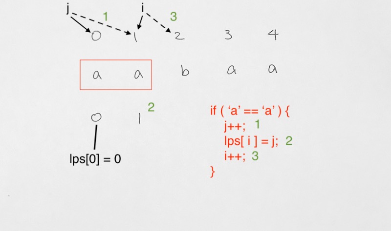
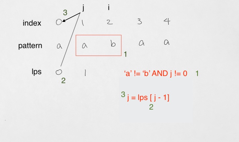
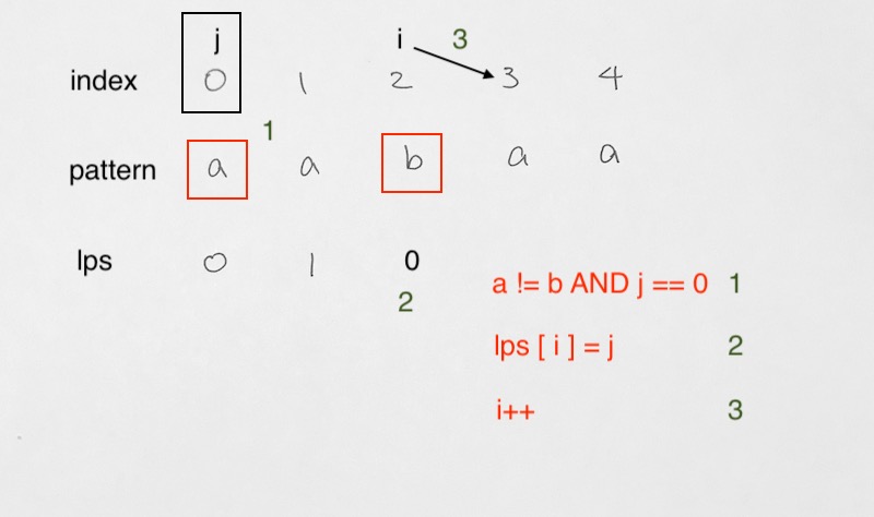
Let’s go through it on a pattern of a a b a a.

We start off j = 0, i = 1. We need to have a parallel matching scheme. Thus, both index will be going down the array in a parallel fashion.
Note that lps[0] is always 0 because at index 0, we only have 1 character.

When going down the array in parallel, we come to 2 situation:

1) Match – we have a match on characters at index i and j. In this case,

1) we move j++ forward
2) and have lps[i] = j;
2) Then, i++.

The i++, j++ is to move the parallel matching forward. The lps[i] = j is so that our lps takes on the j’s index. The reason why we want our lps array to have j as values is because index j is an indicator of how many matches we currently have. i is simply the index of the substring we are checking.

2) Mismatch –

mismatch where j != 0

In this case, we assign j to lps[j-1]. Then compare values at j and i again.

mismatch where j == 0

Here, j has reached back to 0. There is a mismatch at i and thus, lps[i] takes on 0.
We then move i forward and start the parallel matching all over again.

We continue on in the main while loop

while (i < patternLength) {

}

until i has reached the end of the pattern.

Thus, the final result is:

0 1 2 3 4 (index)
a a b a a (pattern)
0 1 0 1 2 (lps)

The KMP matching algorithm

Now that we have the lps array, we can process the KMP algorithm.

First let’s set it up:

let i = 0; // index for txt[]

let j = 0; // index for pat[]

while (i < textLength) {

if (pattern[j] == text[i]) {j++; i++;}

...

}

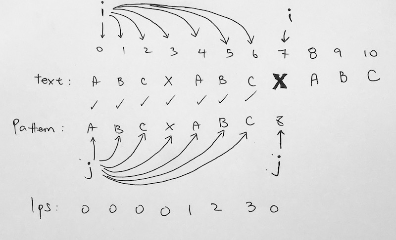
Basically, we have i as the index of text, and j as index of pattern.
If the character of text at index i matches character of pattern at index j, we simply move forward both i and j.

This way, we iterate down both arrays and compare characters in such fashion.

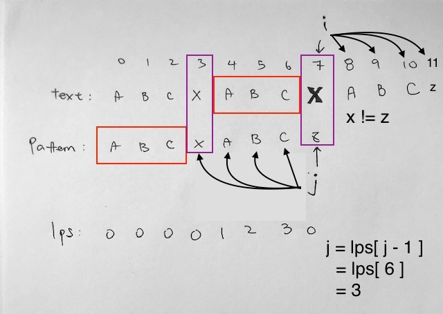
In our example, notice we move down and the characters match up like so: “a b c x a b c..” However, you should think of it as characters match taking place for prefix “abc”, then a substring “x”, then suffix “abc”. Eventually, we hit a mismatch at “x” and “z” at index 7.

A mismatch is when the characters of pattern and text are not equal, AND i is still within the text.length.

(i < textLength && pattern[j] != text[i]) {

...

}

Then we check to see if pattern index j is at 0 or not.
If j is at 0, it means we are at the very beginning of the pattern and cannot go backwards anymore. Thus, we simply have text index i move forward to go on with the next match.

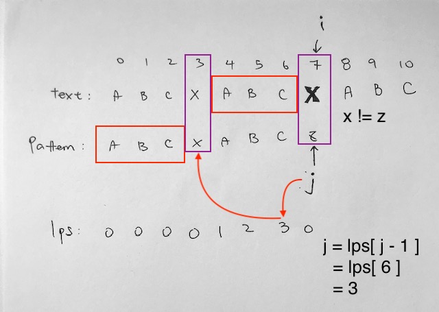
However, if j is not 0, it means, it needs to jump back to a certain point on the pattern. The number of steps to jump back is decided by the lps array at j-1.

if (j != 0)

j = lps[j - 1];

else

i = i + 1;

Now, in the standard Naive way, j comes back to index 0 (the pattern’s beginning). i goes to index 1, then they start comparing again. This is too slow and cumbersome.

The secret to KMP is that we have a Prefix Suffix array that tells us how far back j should jump on the pattern array.

The LPS array will tell j which index to jump so that we don’t have to start from the beginning of the pattern.

The LPS array will have us jump back to a certain niche between two matching substrings, the prefix and suffix.

The reason why we can jump in between the suffix and prefix substring is because on the previous match, we ran through:

prefix + substring1 + suffix
“abc” + “x” + “abc”

The suffix of the previous match (“abc”) matches our current prefix pattern (“abc”). Thus, we always start at the beginning of the substring (“x”).

Let’s continue with our example.

In our previous match, the prefix is “abc”. The substring is “x”. The suffix is “abc”.

Hence, for our next match, we don’t need to match up the prefix again. We already know that the suffix of our previous run is already a match with our current pattern’s prefix of “abc”. Hence we skip that part entirely.

Instead, j just jumps straight to the “x”. In other words, the number of steps to jump back is decided by the lps array at j-1. That is basically how the lps array helps us save steps.

After our index j jumps to index 3, we continue matching.
text[7] = x, pattern[3] = x √
text[8] = a, pattern[4] = a √
…
…

until our index j finally runs to end of the pattern. This signifies that we have a complete pattern match.

We want to see where the index of the match happened in text, so we simply do i – j, which basically means at the last character match at index i, just subtract pattern.length in order to get the index i of where the match starts. In our case, it is i(12) – j(8) = 4.

Boyer Moore (good suffix heuristic)

May 23, 2019algorithms, javascriptadmin

source code – https://github.com/redmacdev1988/boyerMoore/blob/master/index.js

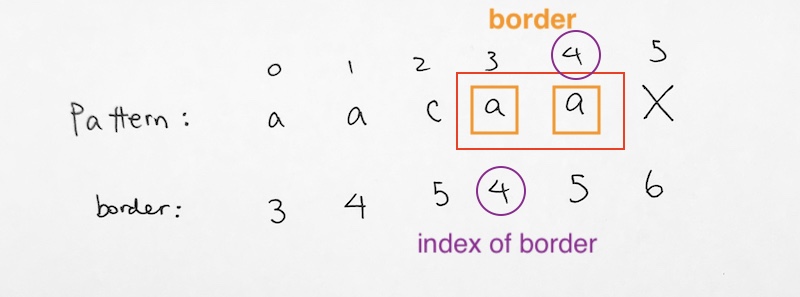
The idea of prefix and suffix borders

A border is a substring which is both proper suffix and proper prefix.

For example, in string ‘ccacc’,’cc’ is a border because it appears in both end of string but ‘cca’ is not a border.

In string, ‘cacc’, ‘c’ is a border because it appears in both end of the string. ‘ca’ is not a border.

Let’s look at example where our pattern is aacaa, and an already calculated Suffix Border Index array.

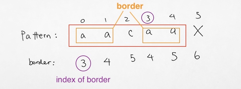
At pattern index 0, we have string aacaa. Its border is aa.
Hence, the prefix border is ‘aa’ at [0][1].
The suffix border is ‘aa’ at [3][4].

We write the beginning index of the suffix border (3) into our border array at index 0.

Thus, for the border array at index 0, we write 3. This means that for the string at pattern index 0, the suffix border starts at index 3.

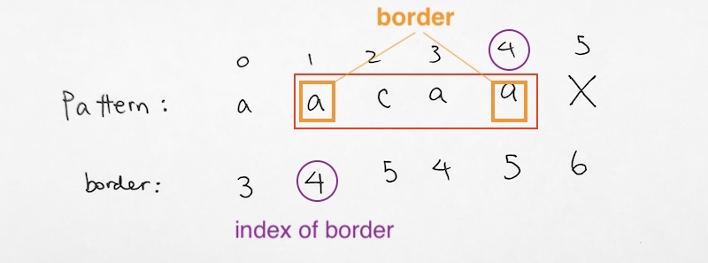
Let’s move on to pattern index 1. We have string acaa. The prefix border is ‘a’ at index 1. The suffix border ‘a’ at index 4.
Hence, for the border array at index 1, we write 4. This means that for the string at pattern index 1, the suffix border starts at index 4.

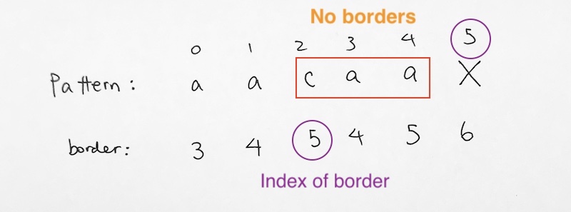
At pattern index 2, we have string ‘caa’. There is no border string. Thus, for the value in our border array, we simply write 5, which represents DNE.

At pattern index 3, we have ‘aa’. The prefix border is ‘a’ at pattern index 3. The suffix border is ‘a’ at pattern index 4. This means that for the string at pattern index 3, the suffix border starts at index 4.

Finally, we come to the last character of pattern index 4 ‘a’. It is only 1 character and does not have any border. So we simply assign the length of the pattern to represent DNE.

How to calculate the Suffix Border Index table

1) to start off, we get the length of the pattern. This value will represent DNE for all the pattern substrings that do not have borders.

2) The idea is that we process it going backwards using two indexes i and j.
We simply have i go backwards. For each i iteration, we get index j and process it to check if the character at i and character at j matches.

3) If it matches, we record a suffix border index. If it doesn’t match, we simply assign it as length of the pattern to designate the suffix index DNE.

i is index of the pattern substring.
j is index of the suffix border.
_borderPosition represents an array that contains all suffix border positions

function processSuffixBorderIndexes() {

let i = _patternLength;

let j = _patternLength+1;

_borderPosition[i] = j;

while (i > 0) {

let p_i = _pattern[i-1];

let p_j = _pattern[j-1];

while (j <= _patternLength && (p_i != p_j)) {

j = _borderPosition[j];

}

i--; j--;

_borderPosition[i] = j;

}

Let’s look at it in detail:

Given pattern ‘aacaa’.

i = 5, j = 6.
border position for 5 is 6, because index 5 does not exist.

0 1 2 3 4 5 (index)
a a c a a X (pattern)
0 0 0 0 0 6 (suffix border index)

We then start going backwards for index i.

i is 5, j is 6

(5 > 0) √
(6 <= 5) X

our j index of 6 is larger than pattern length, so we skip.
decrement i, j to 4, 5.

_borderPosition[4] = 5. This means at pattern index 4, the border index is 5, which denotes DNE. It means the substring at pattern index 4 does not have a border.

0 1 2 3 4 5 (index)
a a c a a X (pattern)
0 0 0 0 5 6 (suffix border index)

i is 4, j is 5

(4 > 0) √
(5 <= 5) √

p[4-1] “a”
p[5-1] “a”

There’s a match so we don’t process index j anymore. We jump out of the loop and decrement i, j to 3, 4.

_borderPosition[3] = 4. This means at pattern index 3, which is substring ‘aa’, the suffix border index is 4.

0 1 2 3 4 5 (index)
a a c a a X (pattern)
0 0 0 4 5 6 (suffix border index)

i is 3, j is 4

(3 > 0) √
(4 <= 5) √

p[3-1] “c”
p[4-1] “a”

There’s no match so we keep processing index j.
We keep processing by going backwards on the _borderPosition array.

j = _borderPosition[4] = 5.

(3 > 0) √
(5 <= 5) √

p[3-1] “c”
p[5-1] “a”

j = _borderPosition[5] = 6.

(3 > 0) √
(6 <= 5) X

skip out of inner while loop
i–; j–; so i is now 2, j is now 5.
_borderPosition[2] = 5.

0 1 2 3 4 5 (index)
a a c a a X (pattern)
0 0 5 4 5 6 (suffix border index)

The substring ‘caa’ at index 2, does not have a suffix border index. So we give is value 5 to denote DNE.

i is 2, j is 5

(2 > 0) √
(5 <= 5) √

Notice j starts over again from the end. The reason we do this is so that we try to find borders. We go back to trying to see if there’s a match for “a”.
if there is, then the current index i has a prefix border.

p[2-1] “a”
p[5-1] “a”

i–;j–‘ 1, 4
_borderPosition[1] = 4;

0 1 2 3 4 5 (index)
a a c a a X (pattern)
0 4 5 4 5 6 (suffix border index)

We then go back one more step to see if there’s additional matches. For every match that happens, we record in the border position of that
match at j.

i is 1, j is 4

(1 > 0) √
(4 <= 5) √

p[1-1] = “a”
p[4-1] = “a”

_borderPosition[0] = 3

0 1 2 3 4 5 (index)
a a c a a X (pattern)
3 4 5 4 5 6 (suffix border index)

Why do we need Suffix borders?

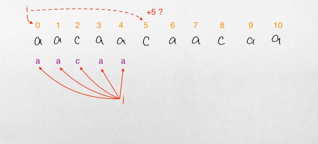
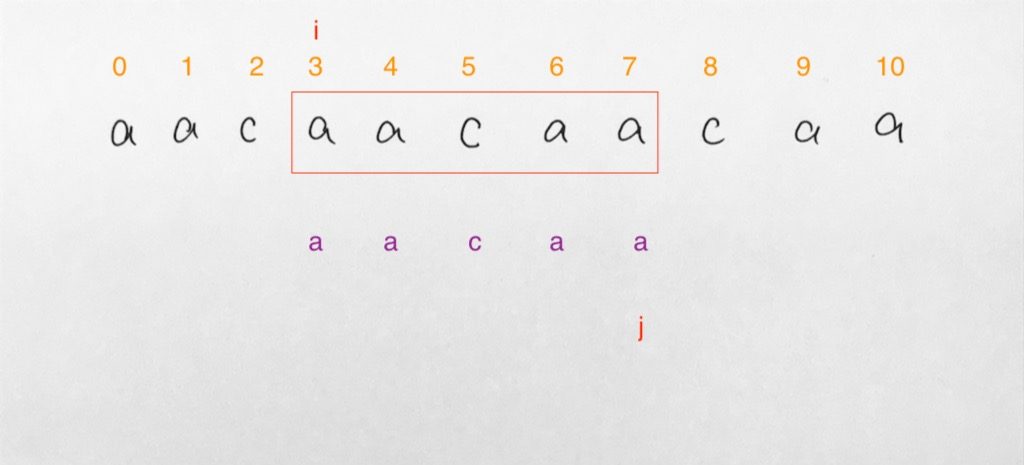
Naive algorithm jumps 1 step at a time. But this is too slow.
Other ways, we jump pattern.length at a time. But we will miss out on potential matches in the middle.

Thus the suffix border array is created so we know where the potential matches are in the middle. WE calculate the suffix border so that we can jump to the correct prefix border for the next potential match.

Setting up the Shift array with Suffix Index Array

So given _borderPositions array as

0 1 2 3 4 5 (index)
a a c a a X (pattern)
3 4 5 4 5 6 (suffix border index)

This means that at index 0 of the pattern, 3 is the index in which the suffix border happens.

Given that if our shift array value is 0, this means it was not assigned.
In this case, we give it the default of the first value of the _borderPositions.

This is so that when we find a match, We know how many steps to skip down. For example, in our case, when a successful search is found, we always skip 3 steps (_shift[0] which is the _borderPosition[0]).

This is so that we can successfully start at the index of the next potential match.

function processShiftIndexes() {

let i;

let j;

j = _borderPosition[0];

for (i = 0; i <= _patternLength; i++) {

// set the border position of first character of pattern to all indices in array shift having shift[i] = 0

if (_shift[i] == 0) _shift[i] = j;

// suffix become shorter than _borderPosition[0],

// use the position of next widest border as value of j

if (i == j) j = _borderPosition[i];

}

After processing, our shift array looks like this:

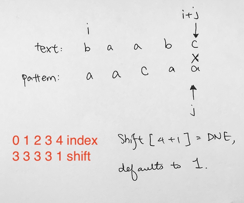
0 1 2 3 4 index
3 3 3 3 1 shift

What this means is that while trying match our pattern char to the text char, if for any reason from index 0 to index 3 is a mismatch, we want our i to shift down 3 spaces. This is because 3 spaces down, there is potential for our pattern to match again due to the suffix border.

However, at index 4, if there’s a mismatch, we only shift i down 1. This is because our very first character is a mismatch so we always need to check for the next one. Also, in our shift array, _shift[4+1] is DNE, so we just use default step 1.

If say, our first character at index 4, matches, then index 3 is a mismatch, we shift i down text array 1 steps because _shift[3+1] = 1.

You can see it with an example like this:

0 1 2 3 4 5 6
b a a c a a b (text)
a a c a a (pattern)

we have a mismatch at index 3 because text[3] “c” != pattern[3] “a”.
Hence we take _shift[j+1] = _shift[4] = 1.

After we shift 1, we get

0 1 2 3 4 5 6
b a a c a a b (text)
_ a a c a a (pattern)

match!

The Search

We do the match going backwards:

i is the index we’re going to use for every substring of the text
j is the index on the pattern. We use this to compare the pattern char to the text char

if the chars at i and j keeps matching, we continue down until j is -1. This means we have matched every character in the pattern matched up in the text.

Thus, when j < 0, we found a pattern match in text. We then log i in order to let the user know where the match happens. Now, we move i down for the next substring to check for a match. So the issue here is, how many steps do we move i down? Typically, we would say, hey why not just shift the i down 5 steps because that's the length of our pattern. We've compared our pattern already, so its safe to go down 5 steps right? The answer is no. What we need to do is shift down 3 steps to the to _shift[0]. This is the 1st of the suffix border index. We need to do this in order to find substring potential matches.

function bmSearch() {

console.log(` ------------------- Now, lets search! --------------------`);

let i = 0;

let j = 0;

while (i <= _textLength - _patternLength) {

console.log(`lets process i ${i}`);

j = _patternLength - 1;

// Keep reducing index j of pattern while characters of pattern and text are matching at this shift s

while ( j >= 0 && _pattern[j] == _text[i+j]) { j--; }

if (j < 0) {

// If the pattern is present at current shift, then index j will become -1 after the above loop

console.log(` √ at ${i}`);

i += _shift[0];

} else {

// pattern at [i] != pattern at [s+j] so shift the pattern shift[j+1] times */

i += (_shift[j+1]) ? _shift[j+1] : 1;

}