ref –
- https://www.geeksforgeeks.org/depth-first-search-or-dfs-for-a-graph/
- https://www.geeksforgeeks.org/breadth-first-search-or-bfs-for-a-graph/
- https://stackoverflow.com/questions/14720691/whats-the-purpose-of-bfs-and-dfs
BFS and DFS are graph search algorithms that can be used for a variety of different purposes. Many problems in computer science can be thought of in terms of graphs. For example, analyzing networks, mapping routes, and scheduling are graph problems. Graph search algorithms like breadth-first search are useful for analyzing and solving graph problems.
One common application of the two search techniques is to identify all nodes that are reachable from a given starting node. For example, suppose that you have a collection of computers that each are networked to a handful of other computers. By running a BFS or DFS from a given node, you will discover all other computers in the network that the original computer is capable of directly or indirectly talking to. These are the computers that come back marked.
BFS specifically can be used to find the shortest path between two nodes in an unweighted graph. Suppose, for example, that you want to send a packet from one computer in a network to another, and that the computers aren’t directly connected to one another. Along what route should you send the packet to get it to arrive at the destination as quickly as possible? If you run a BFS and at each iteration have each node store a pointer to its “parent” node, you will end up finding route from the start node to each other node in the graph that minimizes the number of links that have to be traversed to reach the destination computer.
DFS is often used as a subroutine in more complex algorithms. For example, Tarjan’s algorithm for computing strongly-connected components is based on depth-first search. Many optimizing compiler techniques run a DFS over an appropriately-constructed graph in order to determine in which order to apply a specific series of operations. Depth-first search can also be used in maze generation: by taking a grid of nodes and linking each node to its neighbors, you can construct a graph representing a grid. Running a random depth-first search over this graph then produces a maze that has exactly one solution.
This is by no means an exhaustive list. These algorithms have all sorts of applications, and as you start to explore more advanced algorithms you will often find yourself relying on DFS and BFS as building blocks. It’s similar to sorting – sorting by itself isn’t all that interesting, but being able to sort a list of values is enormously useful as a subroutine in more complex algorithms.
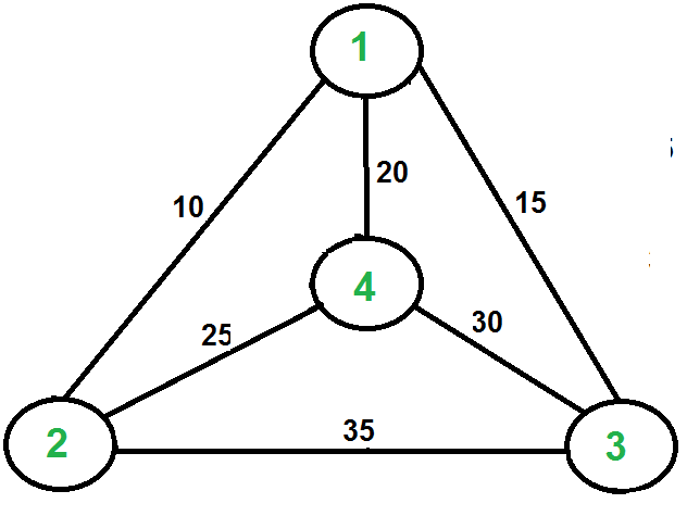
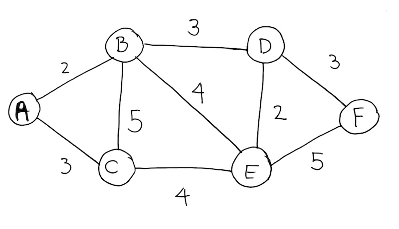
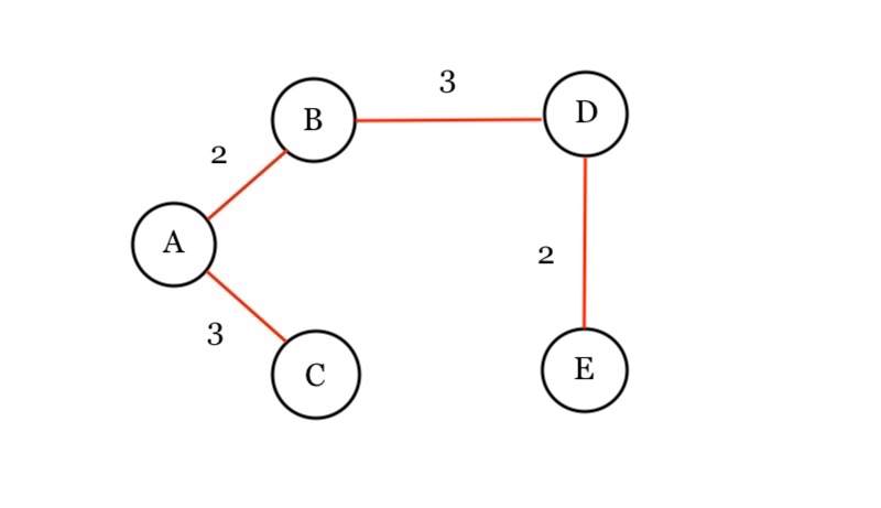
We use graphs to present connected nodes.
Graph consist of nodes and edges.
Adjacent – if two nodes are directed connected. They are neighbors.
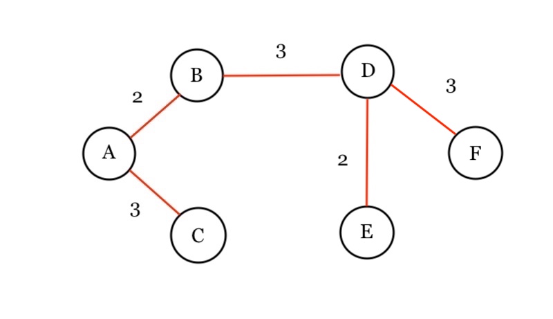
If it’s a directed graph, and John has an arrow towards Bob, then John is adjacent to Bob. But opposite not true.
Edges also have a weight. If two people interact a lot, they can have a higher weighted edge.
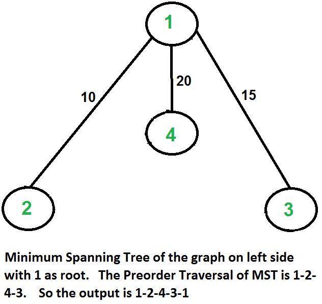
Finding two shortest path to two nodes.
Adjacency Matrix
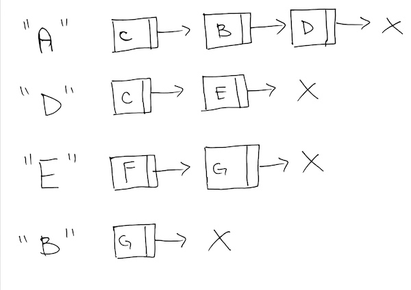
An adjacency list is a collection of unordered lists used to represent a finite graph.
Each list describes the set of neighbors of a vertex in the graph.
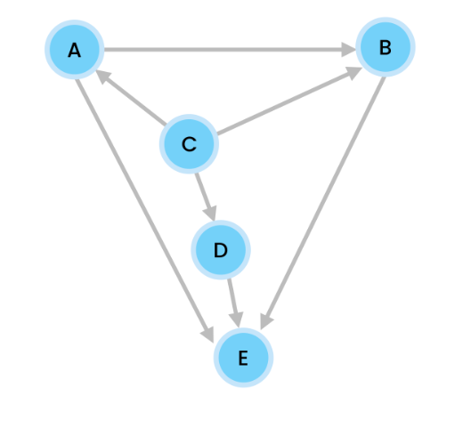
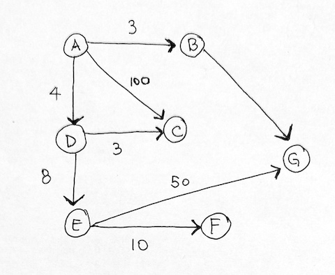
Let’s do Depth First Search on our example graph
The idea is to go forward in depth while there is any such possibility. If not then backtrack.
Whenever we push an unvisited node, we print it.
Before we start, there are two assumptions:
– we start at node C
– nodes are inserted in alphabetical order.
We use a stack.
So we start at C. We push C onto our stack, and print it.
stack: C
output: C
C is connected to three nodes, A, B, and D. We do this alphabetically so we push A onto the stack, and print it.
stack: C A
output: C A
At A, we have two nodes, B and E. We push B onto our stack, and print it.
stack: C A B
output: C A B
B has one neighbor E. So we push E onto the stack, and print it.
stack: C A B E
output: C A B E
Since E has no connecting neighbors, we pop it.
stack: C A B
output: C A B E
We are now at B. B’s only neighbor of E has already been visited so we pop B.
stack: C A
output: C A B E
A’s neighbors B and E have all been visited. So we push A.
stack: C
output: C A B E
Now we’re at C.
C’s A has been visited, and B has also been visited. But B is unvisited so we push D onto the stack, then print it.
stack: C D
output: C A B E D
D has no unvisited nodes so we pop it.
stack: C
output: C A B E D
C has no unvisited nodes so we pop.
stack:
output: C A B E D
Stack is empty so we’re done.
Source Code
We create a list that has a tail pointing to the latest item we insert. That way, everything is order. Whatever you added first, will be processed first as head is referencing it. Tail will always reference the very last item you add.
1 2 3 4 5 6 7 8 9 10 11 12 13 14 15 16 17 18 19 20 21 22 23 24 25 26 27 28 29 30 31 32 33 34 35 36 37 38 39 40 41 42 43 44 45 46 47 48 49 50 51 52 53 54 55 56 57 |
let l = console.log; function Node(data, next) { this.data = data; this.next = next; this.print = function(){ console.log(`Node - ${this.data}`); } } let createLinkedListInstance = (function LinkedList() { let head = null; let tail = null; let iterator = null; return new class LinkedList { add = function(value) { if (!head && !tail) { head = new Node(value, null); tail = head; iterator = head; } else { tail.next = new Node(value, null); tail = tail.next; } } print = () => { for (let tmp = head; tmp != null; tmp = tmp.next) { tmp.print(); } } next = () => { if (iterator) { let tmp = iterator; iterator = iterator.next; return tmp; } else { return null; } } hasNext = () => { return iterator ? true : false; } resetIterator = () => { iterator = head; } } }); |
Create a Graph with x number of nodes.
|
|
let createGraphInstance = (function(numOfVertices) { // private properties let output = []; console.log(`create a graph with ${numOfVertices} nodes`); var numOfNodes = numOfVertices; var adj = []; |
We use recursion on the local stack frame in order to simulate a stack.
Each list that is referenced by an Adj[key] is pushed onto the stack. As we process each node down this list, we get more keys, say key2.
We then push list referenced by Adj[key2] onto the local stack frame by recursively calling the function. We keep doing this until we exhaust this list.
Then the function gets popped off the local stack frame.
1 2 3 4 5 6 7 8 9 10 11 12 13 14 15 16 17 18 19 20 21 |
let _dfsUtil = function(fromNodeKey, visitedArr) { l(`PUSH adj[${fromNodeKey}] onto stack`); output.push(fromNodeKey); visitedArr[fromNodeKey] = true; let list = adj[fromNodeKey]; while (list && list.hasNext()) { let node = list.next(); let nodeKey = node.data; if (!visitedArr[nodeKey]) { _dfsUtil(nodeKey, visitedArr); } else { l(`node ${fromNodeKey} - `, `already processed ${nodeKey}`); } } l(`POP adj[${fromNodeKey}] from stack`); } // |
We look at our graph, and add the neighbors that are connected to our node. We always do this before we run the DFS function.
1 2 3 4 5 6 7 8 9 10 11 12 13 14 15 16 17 18 |
return new class Graph { // public, prototype addEdge = function(fromNodeKey, toNodeKey) { let list = adj[fromNodeKey]; if (!list) { l('creating new'); adj[fromNodeKey] = createLinkedListInstance(); if (toNodeKey) { adj[fromNodeKey].add(toNodeKey); } } else { list.add(toNodeKey); } } // |
After adding all the nodes, and specifying how many nodes we have in the constructor, we are ready to call this function.
|
|
// recursion is the stack dfs(nodeNumber) { l(`starting from node ${nodeNumber}`); let visited = new Array(numOfNodes); _dfsUtil(nodeNumber, visited); } |
print our adjacency list and the lists that they contain
|
|
print = () => { l(`-- printing --`); let allKeys = Object.keys(adj); l(allKeys); for (const key of allKeys) { l(`------ ${key} --------`); adj[key].print(); } } |
print the output array
1 2 3 4 5 6 7 8 9 10 11 12 13 14 15 16 17 18 19 20 21 22 23 24 25 |
printOutput = () => { l(output); } } }); let g = createGraphInstance(5); g.addEdge('a', 'b'); g.addEdge('a', 'e'); g.addEdge('b', 'e'); g.addEdge('c', 'a'); g.addEdge('c', 'b'); g.addEdge('c', 'd'); g.addEdge('d', 'e'); g.addEdge('e'); g.print(); // let's do this starting from node 2 g.dfs('c'); g.printOutput(); |
Breadth First Search on the graph
The trick is that you visit a dequeued node. If that node is NOT visited, we add its neighbors to the queue. If that node HAS ALREADY BEEN visited, we keep dequeueing.
We start at C, so we add C to the queue.
queue: [C]
We remove C from the queue and visit it.
output: C
queue: []
We now must add C’s unvisited neighbors tot he queue (in alphabetical order).
output: C
queue: [A, B, D]
We visit A, and remove it from the queue.
output: C A
queue: [B, D]
Since we visited A, we must add A’s unvisited neighbors to the queue. Those neighbors are B and E.
output: C A
queue: [B, D, B, E]
We visit B, and dequeue it.
output: C A B
queue: [D, B, E]
Since we visited B, let’s look at its neighbors. It has one neighbor E. Let’s add it to the queue.
output: C A B
queue: [D, B, E, E]
No we visit D and print. Then dequeue it.
output: C A B D
queue: [B, E, E].
since we visited D, we must add its unvisited neighbors E.
output: C A B D
queue: [B, E, E, E]
Now we dequeue B, but we see that we have already visited it.
output: C A B D
queue: [E, E, E]
We then dequeue E. It has not been visited so we output it.
output: C A B D E
queue: [E, E]
E has no neighbors so we don’t add anything to the queue.
We then dequeue again. Has no neighbors so we continue to dequeue.
output: C A B D E
queue: [E]
Finally, we dequeue the last E. It has already been printed. And it has no neighbors. The queue is now empty so we’re done.
output: C A B D E
queue: []
We first create a queue.
1 2 3 4 5 6 7 8 9 10 11 12 13 14 15 16 17 18 19 20 21 22 23 24 25 26 27 28 29 30 31 32 33 34 35 36 |
let createQueue = (function Queue() { let head = null; let tail = null; return new class Queue { enqueue = value => { if (!head && !tail) { head = new Node(value, null); tail = head; } else { tail.next = new Node(value, null); tail = tail.next; } } dequeue = () => { let tmp = head; head = head.next; if (!head) { tail = null; } return tmp; } size = () => { let tmp = head; let count = 0; while (tmp) { count++; tmp = tmp.next; } return count; } } }); |
We use the Linked List from the previous example.
So with Breadth first traversal of the graph, the trick is that we start at the initial node.
We then take all the neighbors of that node and add them to the queue. Once we added all those neighbors, we pop the initial node, and then move on to process the next one in queue.
1 2 3 4 5 6 7 8 9 10 11 12 13 14 15 16 17 18 19 20 21 22 23 |
let createBreadthFirstSearchForGraph = (function(numOfVertices) { // private here let output = []; var numOfNodes = numOfVertices; var adj = []; return new class BFSGraph { addEdge = function(fromNodeKey, toNodeKey) { let list = adj[fromNodeKey]; if (!list) { l('creating new'); adj[fromNodeKey] = createLinkedListInstance(); if (toNodeKey) { adj[fromNodeKey].add(toNodeKey); } } else { list.add(toNodeKey); } } // |
So as you can see, we give it an initial key to start from. In our case it is ‘c’. So fromNodeKey is ‘c’.
We then keep track if they are visited or not via a visited array.
Initially, we only have one node in the queue. So we start processing the while loop. We pop the ‘c’ node and then push all the nodes from its neighbors via an inner while loop.
In this inner loop, we check to see if the key has been processed by associative array access on the visited array. If it has not been visited, we mark it visited and then add it onto our queue to be processed later.
1 2 3 4 5 6 7 8 9 10 11 12 13 14 15 16 17 18 19 20 21 22 23 24 25 26 27 28 29 30 31 32 33 34 35 36 37 |
bfs = fromNodeKey => { let visited = new Array(numOfNodes); let queue = createQueue(); visited[fromNodeKey] = true; l(visited); queue.enqueue(fromNodeKey); l(queue); let s; while (queue.size() != 0) { // 2) we then process them one by one // base case is whatever node you want to start from s = queue.dequeue(); output.push(s.data); let list = adj[s.data]; // 1) we push all neighbors of current node onto the queue while (list.hasNext()) { let node = list.next(); let nodeKey = node.data; if (!visited[nodeKey]) { visited[nodeKey] = true; queue.enqueue(nodeKey); } } } } .... .... } }); |
Source Code
Depth First Graph Traversal
1 2 3 4 5 6 7 8 9 10 11 12 13 14 15 16 17 18 19 20 21 22 23 24 25 26 27 28 29 30 31 32 33 34 35 36 37 38 39 40 41 42 43 44 45 46 47 48 49 50 51 52 53 54 55 56 57 58 59 60 61 62 63 64 65 66 67 68 69 70 71 72 73 74 75 76 77 78 79 80 81 82 83 84 85 86 87 88 89 90 91 92 93 94 95 96 97 98 99 100 101 102 103 104 105 106 107 108 109 110 111 112 113 114 115 116 117 118 119 120 121 122 123 124 125 126 127 128 129 130 131 132 133 134 135 136 137 138 139 140 141 142 143 144 145 146 147 148 149 150 151 152 153 |
let l = console.log; function Node(data, next) { this.data = data; this.next = next; this.print = function(){ console.log(`Node - ${this.data}`); } } let createLinkedListInstance = (function LinkedList() { let head = null; let tail = null; let iterator = null; return new class LinkedList { add = function(value) { if (!head && !tail) { head = new Node(value, null); tail = head; iterator = head; } else { tail.next = new Node(value, null); tail = tail.next; } } print = () => { for (let tmp = head; tmp != null; tmp = tmp.next) { tmp.print(); } } next = () => { if (iterator) { let tmp = iterator; iterator = iterator.next; return tmp; } else { return null; } } hasNext = () => { return iterator ? true : false; } resetIterator = () => { iterator = head; } } }); let createGraphInstance = (function(numOfVertices) { // private properties let output = []; console.log(`create a graph with ${numOfVertices} nodes`); var numOfNodes = numOfVertices; var adj = []; let _dfsUtil = function(fromNodeKey, visitedArr) { l(`PUSH adj[${fromNodeKey}] onto stack`); output.push(fromNodeKey); visitedArr[fromNodeKey] = true; let list = adj[fromNodeKey]; while (list && list.hasNext()) { let node = list.next(); let nodeKey = node.data; if (!visitedArr[nodeKey]) { _dfsUtil(nodeKey, visitedArr); } else { l(`node ${fromNodeKey} - `, `already processed ${nodeKey}`); } } l(`POP adj[${fromNodeKey}] from stack`); } // return new class Graph { // public, prototype addEdge = function(fromNodeKey, toNodeKey) { let list = adj[fromNodeKey]; if (!list) { l('creating new'); adj[fromNodeKey] = createLinkedListInstance(); if (toNodeKey) { adj[fromNodeKey].add(toNodeKey); } } else { list.add(toNodeKey); } } // // recursion is the stack dfs(nodeNumber) { l(`starting from node ${nodeNumber}`); let visited = new Array(numOfNodes); _dfsUtil(nodeNumber, visited); } print = () => { l(`-- printing --`); let allKeys = Object.keys(adj); l(allKeys); for (const key of allKeys) { l(`------ ${key} --------`); adj[key].print(); } } printOutput = () => { l(output); } } }); let g = createGraphInstance(5); g.addEdge('a', 'b'); g.addEdge('a', 'e'); g.addEdge('b', 'e'); g.addEdge('c', 'a'); g.addEdge('c', 'b'); g.addEdge('c', 'd'); g.addEdge('d', 'e'); g.addEdge('e'); g.print(); // let's do this starting from node 2 g.dfs('c'); g.printOutput(); |
Breadth First Traversal for Graphs
Linked List used is same as above.
1 2 3 4 5 6 7 8 9 10 11 12 13 14 15 16 17 18 19 20 21 22 23 24 25 26 27 28 29 30 31 32 33 34 35 36 37 38 39 40 41 42 43 44 45 46 47 48 49 50 51 52 53 54 55 56 57 58 59 60 61 62 63 64 65 66 67 68 69 70 71 72 73 74 75 76 77 78 79 80 81 82 83 84 85 86 87 88 89 90 91 92 93 94 95 96 97 98 99 100 101 102 103 104 105 106 107 108 109 110 111 112 113 114 115 116 117 118 119 120 121 122 123 124 125 126 127 128 |
let createQueue = (function Queue() { let head = null; let tail = null; return new class Queue { enqueue = value => { if (!head && !tail) { head = new Node(value, null); tail = head; } else { tail.next = new Node(value, null); tail = tail.next; } } dequeue = () => { let tmp = head; head = head.next; if (!head) { tail = null; } return tmp; } size = () => { let tmp = head; let count = 0; while (tmp) { count++; tmp = tmp.next; } return count; } } }); let createBreadthFirstSearchForGraph = (function(numOfVertices) { // private here let output = []; var numOfNodes = numOfVertices; var adj = []; return new class BFSGraph { addEdge = function(fromNodeKey, toNodeKey) { let list = adj[fromNodeKey]; if (!list) { l('creating new'); adj[fromNodeKey] = createLinkedListInstance(); if (toNodeKey) { adj[fromNodeKey].add(toNodeKey); } } else { list.add(toNodeKey); } } // bfs = fromNodeKey => { let visited = new Array(numOfNodes); let queue = createQueue(); visited[fromNodeKey] = true; l(visited); queue.enqueue(fromNodeKey); l(queue); let s; while (queue.size() != 0) { // 2) we then process them one by one // base case is whatever node you want to start from s = queue.dequeue(); output.push(s.data); let list = adj[s.data]; // 1) we push all neighbors of current node onto the queue while (list.hasNext()) { let node = list.next(); let nodeKey = node.data; if (!visited[nodeKey]) { visited[nodeKey] = true; queue.enqueue(nodeKey); } } } } print = () => { l(`-- printing --`); let allKeys = Object.keys(adj); l(allKeys); for (const key of allKeys) { l(`------ ${key} --------`); adj[key].print(); } } printOutput = () => { l(output); } } }); let b = createBreadthFirstSearchForGraph(5); b.addEdge('a', 'b'); b.addEdge('a', 'e'); b.addEdge('b', 'e'); b.addEdge('c', 'a'); b.addEdge('c', 'b'); b.addEdge('c', 'd'); b.addEdge('d', 'e'); b.addEdge('e'); b.print(); b.bfs('c'); b.printOutput(); |